ANOVA
We return to the issue of central tendency. Often, we want to compare more than one pair of means at a time. We may also wish to compare means across many groups when we control for one or more factors. Regression is another form of this question, asking whether changing one variable affects the mean value of another variable. All these situations lend themselves to an ANOVA (short for ANalysis Of VAriance). Despite its name, ANOVA is usually applied to understanding differences in central tendency. It gets its name because it uses variance to address questions about the mean.
How an ANOVA works
A thought model helps to understand how an ANOVA works. Suppose we have a factor that lets us divide our data into several groups (called treatments). For example, if we grew plants under several types of fertilizer, fertilizer would be considered a factor, and each type of fertilizer would represent a treatment. Factors are categorical variables; in other words, they are nominal or ordinal data.
Let’s also suppose that all the groups come from populations with the same variance, although the means of those populations might be different. If the means of the individual groups are equal, the total variation of all the groups combined will not be greater than the variation within any group. However, if at least one of the groups has a different mean, the total variance will be greater than the variance of any of the groups. This is similar to what an ANOVA does: by comparing variance within and among groups, an ANOVA can test whether the means of the groups differ. An ANOVA uses an F-test to evaluate whether the variance among the groups is greater than the variance within a group.
Another way to view this problem is that we could partition the variance, that is, we could divide the total variance in our data among multiple sources of that variation. Some variance would come from variation among replicates within each group. Some variance may also come from differences among the groups. Partitioning variance is an incredibly important concept within statistics. For scientists, it is a useful way of looking at the world: variation is everywhere, and we want to know the relative contributions of all the sources of variation. Moreover, we should focus first on the most important sources of variation.
An ANOVA makes three assumptions. First, the population must be randomly sampled. Second, each population must be normally distributed. Third, all the populations must have the same variance, that is, they must be homoscedastic. As with all tests, you must demonstrate that these are valid assumptions before performing an ANOVA.
The null hypothesis of an ANOVA is that the means of all the populations are equal, with the alternative hypothesis being that at least one of the means is different. Unlike other statistical methods, ANOVA is generally not used for creating confidence intervals. ANOVA is nearly always a p-value approach in which one tests a null hypothesis, specifically that the mean values of all the groups (treatments) are the same (often called the zero-null hypothesis). We will have to follow the ANOVA with additional analyses to get the effect size, which should always be our ultimate goal.
One-way ANOVA: testing for one factor
The simplest type of ANOVA is called a one-way ANOVA. We use a one-way ANOVA when we have a single factor or explanatory variable. For example, we may have measured the weight percent of strontium in three groups of rocks: basalt, andesite, and rhyolite. We would want to test whether the mean weight percent of strontium is the same for all three rock types.
In a one-way ANOVA like this, we have two potential sources of variation: among-groups and within-group. The variation among the groups is called the explained variation because rock type will be the factor that accounts for this variation. We also have the variation within the groups, that is, variation among the replicates within each type of rock, which is called the unexplained variation. It is unexplained in that we cannot identify what produces that variation. For example, we might see that strontium varies among rhyolites, but we do not know why, at least from this data.
ANOVA results are presented in a standard table format. You should become comfortable with interpreting any ANOVA table.
Analysis of Variance Table Response: strontium Df Sum Sq Mean Sq F value Pr(>F) rocktype 2 2.8350 1.4175 1.4392 0.2753 Residuals 12 11.8189 0.9849
The first column in an ANOVA table lists the sources of variation, with a row for the explained variation (the among-group variation, also called among-treatments variation), here called rocktype. Below that is a row for the unexplained variation (the within-group variation, also called among-replicates variation), here labeled Residuals. Although R omits it, many ANOVA tables add a third row at the bottom that shows the total variation.
The second column (Df) is the degrees of freedom. In a one-way ANOVA, there are m-1 degrees of freedom for the among-group (explained) variation, where m is the number of groups. There are N-m degrees of freedom for the unexplained (within-group) variation, where N is the total number of observations equal to m x n (provided all the groups have the same sample size, n). These sum to produce N-1 total degrees of freedom, although R does not report this in the ANOVA table.
The third column (Sum Sq) is the sum of squares for each source of variation. The sum of squares is the sum of the squared deviations of each observation from the mean. For the among-groups row, this is the mean of each group compared to the mean of all the data. For the within-groups row, this is each observation in a group compared to the mean of that group. Adding the sums of squares in the first two rows produces the total sum of squares, again, not shown in R.
The fourth column (Mean Sq) is the mean squares, calculated by dividing the sum of squares by the degrees of freedom within each row. This is therefore a column of variances. The first row is the among-group variance, and the second row is the within-group variance. One could do this for the total row (again, not shown) to calculate the total variance among all the data.
The fifth column (F value) is the F-ratio, with the among-group variance in the numerator and the within-group variance in the denominator. Understanding this F ratio is critical for understanding how an ANOVA works. If there are no differences among groups, the among-group variance will estimate the within-group variance, so their ratio should be close to one. If the means of the groups are different, then the among-group variance will be larger, causing the ratio to exceed one. In an ANOVA, the F-test is a one-tailed (right-tailed) test because we expect the ratio to be close to one if the null hypothesis is true and greater than one if the null hypothesis is false.
R and some other programs add a sixth column (Pr(>F)) that lists the p-value for the F-ratio. This value is the probability of observing an F statistic equal to or larger than the observed F statistic if the null hypothesis is true. Remember as always that a p-value is a probability of our data (if the null hypothesis is true), not a probability of whether the null hypothesis is true.
An example
We will use a data set on air quality to demonstrate an ANOVA. In this data set, a pollutant was measured multiple times (replicated) in three cities. As usual, we import the data and run str() to see the variables and their format. To make things easier by avoiding $ notation, we attach() the data frame to simplify accessing the variables.
airQuality <- read.table(file="airQuality.txt", header=TRUE, sep=",") str(airQuality) attach(airQuality)
Preliminary steps: check the assumptions of ANOVA
We should always visualize our data first, partly so that we can evaluate the assumptions of the test. In this case, the assumptions are random sampling, normally distributed data within each group, and equal variances among the groups. Knowing that we had a good sampling design that avoided pseudoreplication is how we can evaluate the first assumption. A strip chart is useful for evaluating the second and third assumptions.
stripchart(pollutant ~ city, pch=16, frame.plot=FALSE)
Calling stripchart() this way will create a row of pollutant values for each city. Read pollutant ~ city as “pollution as a function of city”; we will use this syntax more when we learn regression.
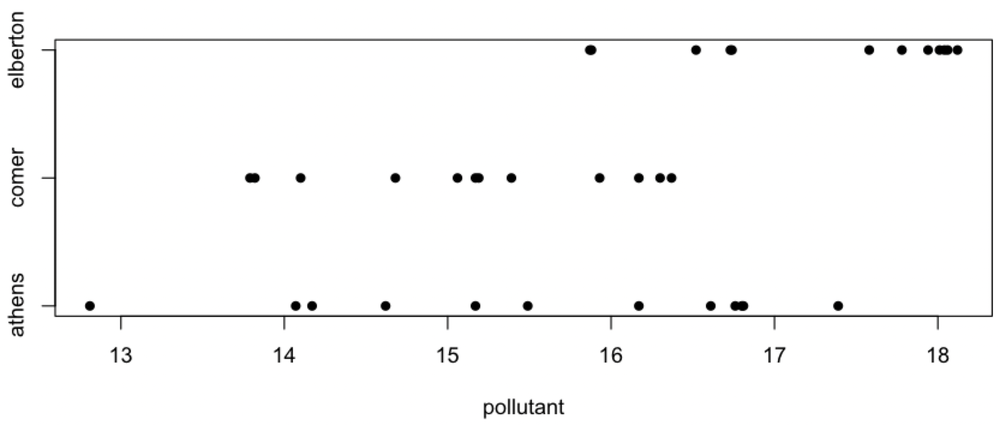
Notice that the data at Elberton might be left-skewed, and this might be cause for caution, but the sample size is small. The variation at Athens appears greater than at Elberton or Comer, so we should test for homoscedasticity, as that is an assumption underlying ANOVA. Therefore, we precede our ANOVA with a Bartlett’s test to verify that the variances of the three groups are indistinguishable, given the amount of data that we have.
bartlett.test(pollutant, city)
Bartlett test of homogeneity of variances data: pollutant and city Bartlett's K-squared = 3.1804, df = 2, p-value = 0.2039
The Bartlett test is not statistically significant (Bartlett’s K-squared = 3.2, df = 2, p-value = 0.20), meaning we cannot detect a difference among the variances. Note the wording, that we cannot detect a difference. The variances in the three populations are almost assuredly different at some degree of precision, meaning that the null hypothesis is false. As such, the p-value tells you only whether you have enough data to detect the difference, a difference that might be trivial and unimportant, yet statistically significant if the sample size is large enough.
With the stripchart and Bartlett’s test, we have shown that the assumptions of the ANOVA are valid (random sampling, normal distribution, equal variances), so we can legitimately perform an ANOVA.
Running the ANOVA
Although there are several ways in R to perform an ANOVA, we will first use the aov() function followed by summary() to show the results. This approach is the most informative.
pollutionANOVA <- aov(pollutant ~ city) summary(pollutionANOVA)
The ANOVA output follows the standard format:
Df Sum Sq Mean Sq F value Pr(>F)
city 2 30.01 15.004 12.41 9.59e-05 ***
Residuals 33 39.90 1.209
---
Signif. codes: 0 '***' 0.001 '**' 0.01 '*' '0.05 '.' 0.1 ' ' 1
The results are statistically significant (F=12.4, df=2, 33, p=9.6e-5), meaning we can reject the null hypothesis that the means of all groups are the same.
For convenience in spotting statistically significant results, R will often tag p-values that meet common thresholds with asterisks, and this key is shown at the bottom. p-values less than 0.001 get three stars, those between 0.001 and 0.01 get two stars, and so on. You will often find p-values tagged this way in the literature, but avoid thinking that there is anything special about these arbitrary cutoffs.
Avoiding attach()
Many functions in R provide a way to avoid using attach() by passing the data frame to an argument called data. For these pollution data, you could skip attaching the data and the risks that attach()entails by adding the data argument:
modelAir <- aov(pollutant ~ city + time, data=airQuality)
Effect size
Our ANOVA let us reject the null hypothesis that the means of the three groups are identical. However, the means of any three groups are almost assuredly different at some level of precision, meaning that the null hypothesis is false. In that case, the p-value tells you only whether you have collected enough data to detect a difference in the means. In this case, the difference in means is detectable, even with our relatively small sample size.
That is not especially helpful. Running an ANOVA did not tell us how much the city controls the pollution level, that is, how much of the variance in pollution arises from differences among the cities. It also doesn’t tell us which of the cities are different, what their mean pollution levels are, or what our uncertainty in those pollution levels is. These are the questions that interest us most, not whether our sample size is large enough to detect a difference, a difference that is quite possibly so small as to be unimportant. To answer these questions that we are truly interested in, we need to measure the effect size.
For an ANOVA, there are three ways to evaluate effect size: η2, confidence intervals on the means, and Cohen’s d. Each tells us something slightly different about the data. The three are complementary, and you will usually calculate more than one of them.
η2
The first approach, η2 (eta-squared, pronounced AY-tuh, or EE-tuh if you’re a Brit), is perhaps the easiest way to measure effect size. It measures the proportion of variance explained by the treatment (in this case, the city). It follows the same idea as r2 and the coefficient of determination in regression.
η2 is the explained sum of squares divided by the total sum of squares, and the ANOVA table reports the sums of squares. Although R’s ANOVA table doesn’t report the total sum of squares, it is just the sum of the values in the sum of squares column. In our example, η2 is therefore 30.01 / (30.01 + 39.90), or 0.43.
Because the various sums of squares add to make the total, η2 must range from 0 (when the treatment sum of squares is zero) to 1 (when the treatment sum of squares equals the total sum of squares). In other words, η2 measures the proportion of variation explained by the treatment. In our example, the city reflects 43% of the variation in pollution, and the proportion of variance that is unexplained is 39.90 / (30.01 + 39.90), or 0.57, so there are other important sources of the variation in pollution.
This manual approach is sufficient when examining a published ANOVA table, but calculating η2 directly from the values in an ANOVA table is more precise and less error-prone. This is easily done in a few steps:
anovaTable <- summary(pollutionANOVA)[[1]] ss <- anovaTable[ , "Sum Sq"] eta2 <- ss / sum(ss) names(eta2) <- trimws(rownames(anovaTable)) eta2
The summary() function in the first line returns a list of ANOVA tables, each stored as a data frame. As only one table is produced in this ANOVA, we extract the first element from the list. In the second line, we extract the sum of squares from this data frame. η2 is calculated in the third line, and the names of the terms are added in the fourth line to make the results more easily interpretable. The trimws() function removes the white space from the ends of the names.
Focus on effect size (η2) when describing the results of an ANOVA by leading with η2 and following with the p-value. Here, you might report something like “Pollution values are strongly tied to the city (η2=0.43, p=9.6e-5)” or “The city explains 43% of the variation in pollution (η2=0.43, p=9.6e-5).”. If you have a table that reports the results of multiple ANOVAs, report η2 in one column, followed by the p-value in another column; do not just report the p-values. In your discussion section, focus on η2 and not the p-value, because the p-value tells you only whether you collected enough data to detect a difference among the treatments.
Confidence intervals on the means
Although η2 is useful, it doesn’t tell us which city or cities are different from the others or by how much. To know that, we need to calculate confidence intervals on each possible pair of means. This is called a pairwise t-test, not to be confused with a paired t-test.
Calculating these is easily done with Tukey’s Honestly Significant Difference (HSD). To run this, we pass the ANOVA object and the grouping variable (in quotes) to the TukeyHSD() function.
TukeyHSD(pollutionANOVA, "city")
The results look like this:
Tukey multiple comparisons of means 95% family-wise confidence level Fit: aov(formula = pollutant ~ city) $city diff lwr upr p adj comer-athens -0.4083333 -1.5098958 0.6932292 0.6381658 elberton-athens 1.7000000 0.5984375 2.8015625 0.0017321 elberton-comer 2.1083333 1.0067708 3.2098958 0.0001304
The output reports estimates of the differences in means (diff) for each pair of cities and the corresponding lower (lwr) and upper (upr) 95% confidence limits on the difference of means. A p-value (p adj) is also listed for each pair, testing whether that difference of means is non-zero (i.e., whether the difference is detectable). This is an adjusted p-value in that it corrects for the fact that there are multiple tests; this keeps the overall type 1 error rate at 0.05. Recall that you could also evaluate statistical significance (i.e., whether the difference is detectable) for each row by seeing whether the confidence interval brackets zero (the null hypothesis of no difference in means). Note that R reports far too many significant figures, so that if you included these results in a paper, you would reduce the number of significant figures to be in line with the data.
From the confidence intervals and the p-values, we can see that Elberton and Comer have detectably different mean values (p=0.00013), as do Elberton and Athens (p=0.0017). Athens and Comer are not distinguishable (p=0.64) given the sample size. Note that the estimates of the difference in means and their confidence limits are reported in the output of TukeyHSD()as the mean of the first city minus the second city. For example, Comer has a smaller mean than Athens, so the difference is negative, whereas the positive difference for Elberton and Athens indicates that the mean is greater for Elberton than Athens.
Cohen’s d
Pairwise t-tests tell us how much pollution differs among the cities in the same units that pollution was measured, and this is a useful and intuitive way of expressing the results. Sometimes, though, we would like to report this with a dimensionless number to provide a metric easily interpreted regardless of whether we have an intuition for the units used in measuring the variable (for example, we do not even know the units of “pollutant” in this study).
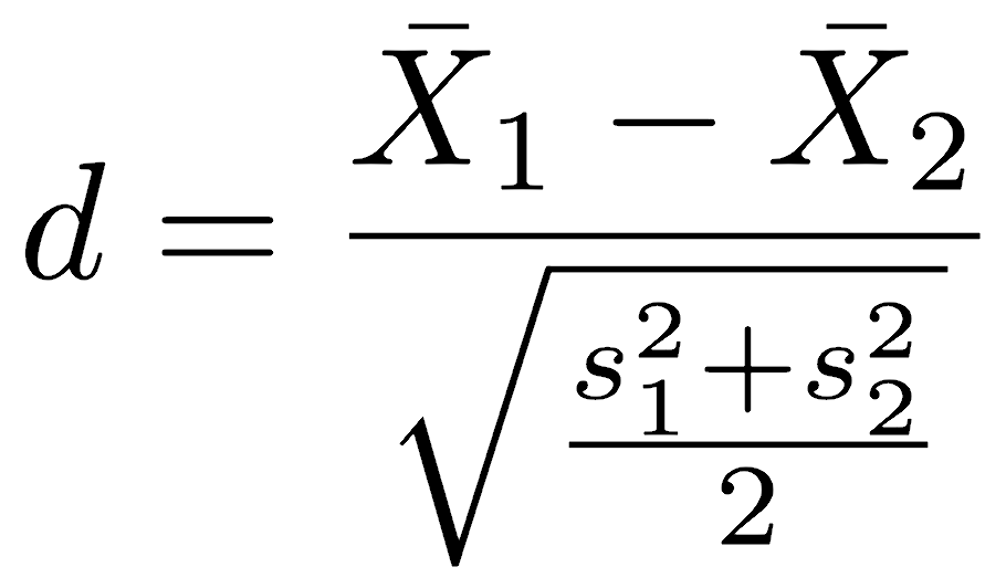
Cohen’s d provides such a dimensionless number, and it is the difference in means scaled by the average standard deviation.
Calculating this is straightforward, even if verbose, and we’ll use comer vs. athens to demonstrate.
athens <- city == "athens" comer <- city == "comer" mean1 <- mean(pollutant[athens]) mean2 <- mean(pollutant[comer]) var1 <- var(pollutant[athens]) var2 <- var(pollutant[comer]) cohensD <- (mean1 - mean2) / sqrt((var1 + var2) / 2) cohensD
Following this procedure for every pair of cities (not shown), Cohen’s d for comer and athens is -0.34, for elberton and athens is 1.45, and for elberton and comer is 2.34. These values are in units of standard deviations, so the difference between elberton and comer is the greatest at 2.34 standard deviations. This matches the strip chart we made initially, where the values of elberton are different and non-overlapping. Cohen’s d is useful in that it gives a dimensionless way of describing the difference in pairs of treatment cases. Note, however, that it provides no estimate of uncertainty (that is, no confidence interval).
Which to use
With three approaches to effect size, the question of which to use will depend on what you would like to know. If you are interested primarily in how much explanatory power the treatment has (city in this case), use η2. If you want to know how much each city differs from the others, along with a measure of the uncertainty in that difference, report the confidence intervals on the mean. If you want a standardized expression of the difference between the treatment cases and don’t need an estimate of the uncertainty in that difference, use Cohen’s d. You will often be interested in more than one of these measures of effect size.
A second way to perform an ANOVA
A second way to run an ANOVA is by combining the anova() and lm() functions. The lm() function stands for linear model, which will play a major role when we discuss regression.
anova(lm(pollutant ~ city))
The generates an ANOVA table identical to the aov() approach. You can still calculate η2 and Cohen’s d, but you cannot run TukeyHSD(). Pairwise t-tests would need to be run instead, and this can be laborious when there are many treatment groups.
A third way to perform an ANOVA
A third way of running a one-way ANOVA is the Welch test, which relaxes the assumption of equal variances in all the groups. The Welch test is run with the oneway.test() command, with the same syntax as the anova() and aov() commands.
oneway.test(pollutant ~ city)
This approach reports the F statistic, degrees of freedom, and p-value, but no ANOVA table, so it provides less insight.
Because the ANOVA table is not reported, you cannot easily calculate η2. You also cannot calculate pairwise confidence limits on the mean with TukeyHSD(), and you would have to run the pairwise t-tests manually. oneway.test() is the least useful of the three approaches because there is no simple way to calculate effect size, and this is a problem because effect size is what you are most interested in.
Two-way ANOVA: testing for two factors
We use a two-way ANOVA when we have two factors for our data. For example, our pollution data has two potential sources of variation — city and time of day — giving us two factors. Variation within any of our factor combinations (a specific time of day for a particular city) is a third source, which is unexplained variation. The two-way ANOVA makes the same assumptions as a one-way ANOVA.
There are two versions of the two-way ANOVA. The simpler version assumes that there is no interaction effect, that variation in one factor (e.g., city) does not change with respect to the other factor (e.g., time of day). The more complicated version allows for interactions between the factors, such as the time of day having a different effect in some cities than in others. One example of this might be that the pollutant doesn’t vary with time of day in small cities, but it does in large cities. You can test for interactions between factors only if you have replicates for each of your factor combinations; that is, you must have replicates for every combination of region and rock type.
For a two-way ANOVA, you need to have a balanced design: the same sample size for each factor and combination of factors. Results from unbalanced designs can be hard to interpret. Balanced design is less of an issue for one-way ANOVA, but it is critical for two-way and multiway ANOVA. Imbalanced designs often result from collecting data before planning data analysis methods or from serious setbacks during data collection that prevent you from collecting the data you planned. Small departures from balanced design may not be a substantial concern, but large departures are.
Think about your statistical analysis when you design the project: if you know that you will use ANOVA, plan to collect the same number of replicates for every combination of city and time of data. Avoid pseudoreplication.
Running a two-way ANOVA is similar to a one-way ANOVA, except that the linear model is pollutant as a function of city and time. The plus sign ( + ) indicates that there is no interaction term. Read this model as “pollutant as a function of city and time”, not city plus time.
pollutionANOVA <- aov(pollutant ~ city + time) summary(pollutionANOVA)
The interaction effect can be included by replacing the plus sign with an asterisk ( * ). Read this model as “pollutant as a function of city and time and their interaction”, not as city times time.
pollutionANOVA <- aov(pollutant ~ city * time) summary(pollutionANOVA)
Running the two-way ANOVA with the interaction term produces a familiar ANOVA table. The main difference is that there are now rows for each source of explained variation, including any interactions. Each source of explained variation has an F-ratio and p-value, as there are now multiple hypotheses being tested.
Df Sum Sq Mean Sq F value Pr(>F) city 2 30.01 15.004 11.576 0.000188 *** time 1 0.52 0.521 0.402 0.530948 city:time 2 0.50 0.250 0.193 0.825474 Residuals 30 38.88 1.296 --- Signif. codes: 0 '***' 0.001 '**' 0.01 '*' '0.05 '.' 0.1 ' ' 1
In this case, the city is a statistically significant source of variation in pollutants (F=11.6, df=2,30, p=0.00019), but the time of day is not (F=0.40, df=1,30, p=0.53); in other words, the variation among cities is detectable, but the variation among time of day is not. The interaction term is not statistically significant either (F=0.19, df=2,30, p=0.83), meaning there is no detectable interaction between specific combinations of city and time.
Effect size: proportion of variance that is explained, via η2
The first way of evaluating effect size is η2, which will tell us the proportion of variance explained by city, by time, and by the interaction of city and time. Combining the several steps described above, it is calculated this way:
anovaTable <- summary(pollutionANOVA) round(anovaTable[[1]]$"Sum Sq" / sum(anovaTable[[1]]$"Sum Sq"), 3)
which returns the following:
1] 0.429 0.007 0.007 0.556
This tells us that city accounts for 43% of the variance (as we saw above), that time of day and the interaction of time and city each account for less than 1% of the variation, leaving 56% of the variance unexplained (i.e., the Residual variance). In other words, the city is an important predictor of pollution, but time and its interaction with the city are not. Most of the variance is still unexplained, which means that we need to consider what other variables might control pollution and test for them.
Effect size: differences among treatments, with confidence intervals
TukeyHSD() can also be called on a two-way ANOVA by supplying a vector of factors in quotes. Note how the interaction term is specified with a colon.
TukeyHSD(pollutionANOVA, c("city", "time", "city:time"))
The output is voluminous, increasing with the number of factors, especially if there is an interaction term. Here, over half of the output focuses on every possible interaction (all 15 of them!). As before, each row provides an estimate of the difference in means for every treatment level (group) within a factor and a confidence interval on the difference in means. The p-value tests for a difference of zero in the means; as always, it tells you whether a difference in means was detectable.
Tukey multiple comparisons of means 95% family-wise confidence level Fit: aov(formula = pollutant ~ city * time) $city diff lwr upr p adj comer-athens -0.4083333 -1.5541171 0.7374504 0.6577398 elberton-athens 1.7000000 0.5542162 2.8457838 0.0027083 elberton-comer 2.1083333 0.9625496 3.2541171 0.0002474 $time diff lwr upr p adj morning-evening 0.2405556 -0.5344521 1.015563 0.5309479 $`city:time` diff lwr upr p adj comer:evening-athens:evening -0.3150000 -2.3141907 1.684190729 0.9965545 elberton:evening-athens:evening 1.9833333 -0.0158574 3.982524062 0.0528044 athens:morning-athens:evening 0.4916667 -1.5075241 2.490857396 0.9739666 comer:morning-athens:evening -0.0100000 -2.0091907 1.989190729 1.0000000 elberton:morning-athens:evening 1.9083333 -0.0908574 3.907524062 0.0680536 elberton:evening-comer:evening 2.2983333 0.2991426 4.297524062 0.0169416 athens:morning-comer:evening 0.8066667 -1.1925241 2.805857396 0.8201390 comer:morning-comer:evening 0.3050000 -1.6941907 2.304190729 0.9970411 elberton:morning-comer:evening 2.2233333 0.2241426 4.222524062 0.0224139 athens:morning-elberton:evening -1.4916667 -3.4908574 0.507524062 0.2377338 comer:morning-elberton:evening -1.9933333 -3.9925241 0.005857396 0.0510200 elberton:morning-elberton:evening -0.0750000 -2.0741907 1.924190729 0.9999970 comer:morning-athens:morning -0.5016667 -2.5008574 1.497524062 0.9716069 elberton:morning-athens:morning 1.4166667 -0.5825241 3.415857396 0.2877627 elberton:morning-comer:morning 1.9183333 -0.0808574 3.917524062 0.0658185
Although no asterisks for p-value thresholds are provided in this table, they would be helpful for quickly scanning the table to identify statistically significant (i.e., non-zero, detectable) differences in means. The only statistically significant differences in pollutants are elberton vs. athens and elberton vs. comer (top table). Time of day does not have a statistically detectable difference in pollutant (middle table). Only two of the interactions generated a statistically detectable difference in pollutant values (bottom table): evenings in Elberton and Comer (p=0.017), and morning in Elberton vs. evening in Comer (p=0.022). Four other combinations have p-values close to 0.05, that is, they are nearing the limit of detectability.
Cohen’s d is not shown, given the laboriousness of the calculations. That, as they say, is an exercise left to the reader.
An alternative way towards a two-way ANOVA
Two-way ANOVAS can also be run with the combination of anova() and lm():
anova(lm(pollutant ~ city + time)) anova(lm(pollutant ~ city * time))
Multiway ANOVAs
ANOVAs can also be run when there are more than two factors, and these are called multiway ANOVAs. Achieving balanced design becomes increasingly difficult as the number of factors increases. Consult a reference text on ANOVA for approaches to this problem and more complicated ANOVA designs.
Multiway ANOVAs can be performed with aov() and anova(lm()). The output from TukeyHSD() may be staggering, especially if there are interaction terms.
Regression ANOVA
You can perform an ANOVA on a regression, with the regression being the source of explained variation and scatter around the line being the unexplained source of variation. You can think of this as a variation of a one-way ANOVA, but instead of having discrete groups, variation arises continuously.
The ANOVA for a regression will report an R-squared value called the Coefficient of Determination, analogous to η2. This is the ratio of the regression sum of squares to the total sum of squares; the latter is not actually shown in the table. This is also equal to the correlation coefficient squared.
The ANOVA for a regression also reports an Adjusted R-squared. Since R-squared always increases as you add regressors (independent variables), an increase in R-squared does not necessarily tell you that additional variables improve the model. The corrected R-squared includes a penalty for additional parameters so that an increase in R-squared is informative: it increases only if the additional parameter explains more variation than expected by chance. Report R-squared when you want to convey the percentage of explained variation. Report the adjusted R-squared when comparing models that have different numbers of independent variables.
ANOVA: a final comment
ANOVA is a common statistical test, but be aware that investigators commonly only report the p-value, leaving the most important part (effect size) unstated or even uninvestigated. Even so, if an ANOVA table is reported, η2 can be easily calculated. Without the data, confidence intervals on the mean and Cohen’s d cannot be calculated.
By not reporting effect sizes, investigators fall into the trap of equating a low p-value (i.e., a statistically significant result) with a scientifically meaningful result. This is particularly true when the sample size is large, allowing them to detect that two means are demonstrably different (that is, the difference in means is not zero), when the difference in means is still very small. Watch for this; it is an extraordinarily common mistake.
Avoid this in your research by not just calculating effect sizes, but emphasizing them in your interpretation of the results. Remember, all an ANOVA p-value tells you is whether the difference in means is detectably non-zero. With enough data, you can detect any difference in means, even ones that are not large enough to be important. By itself, a p-value is not very interesting.
The non-parametric Kruskal–Wallis and Friedman tests
The Kruskal–Wallis and Friedman tests are two common non-parametric alternatives to ANOVA, and they are commonly invoked when the data are not normally distributed, a key assumption of ANOVA. Like many non-parametric tests, the Kruskal–Wallis and Friedman tests are performed on ranks and are therefore far less influenced by outliers. The use of ranks, however, leads to a considerable loss of power. Both tests assume random sampling.
The Kruskal–Wallis test is used for one-way analysis of variance. It is performed in R with the kruskal.test() function, with a model-formula syntax.
kruskal.test(pollutant ~ city)
Two-way non-parametric analysis of variance is performed with the friedman.test() function. No replicates are permitted with the Friedman test. The code below is an example of how to perform a Friedman test in R, although it returns an error with this particular data set because of the replicates.
friedman.test(pollutant ~ city | time)
Background reading
Read Chapter 6 on comparing two samples, performing the code as you read. Focus for now on the t-test, wilcox, and paired-sample pages at the beginning of the chapter. We will not cover the binomial test, the chi-square contingency test, or Fisher’s exact test, but be aware that these exist if you should need them later. The binomial test is useful when comparing proportions, and the chi-square and Fisher’s exact tests are useful when comparing contingency tables. Contingency tables report counts of cases under different combinations of factors; for example, you could make a 2x2 contingency table of master’s vs. Ph.D. degrees for women and men. The null hypothesis would be that the two factors are unrelated.
