Discriminant Function Analysis
DFA is a multivariate technique for describing a mathematical function that will distinguish among predefined groups of samples. As an eigenanalysis method, DFA has a strong connection to multiple regression and principal components analysis. In addition, DFA is the counterpart to ANOVA and MANOVA: in DFA, continuous variables (measurements) are used to predict a categorical variable (group membership), whereas ANOVA and MANOVA use a categorical variable to explain variation in (predict) one or more continuous variables. Two examples help to show how DFA can be useful.
For the first example, suppose you have a series of morphological measurements on several species and want to know how well those measurements allow those species to be distinguished. One approach would be to perform a series of t-tests or ANOVAs to test for differences among the species, but this would be tedious, especially if there are many variables. Another approach might be a principal components analysis to see how the groups plot in multidimensional space, and this is often a good exploratory approach. DFA takes a similar approach to PCA, but DFA seeks a linear function that maximizes group differences. The function will show how well the species can be distinguished, as well as where the classification is robust and where it may fail.
In the second example, suppose you are studying ancient artifacts that are thought to have come from a set of mines. You have collected a set of rock samples from those mines and made consistent geochemical measurements on those samples. You have also made those measurements on the artifacts. DFA can be used to find a function that uses your geochemical measurements to separate your samples into the mines from which they came. That function can then be applied to the artifacts to predict which mine was the source of each artifact.
How it works
There are several types of discriminant function analysis, but this lecture will focus on classical (Fisherian, yes, it’s R.A. Fisher again) discriminant analysis or linear discriminant analysis (LDA), which is the most widely used. In the simplest case, there are two groups to be distinguished. LDA will find an equation that maximizes the separation of the two groups using the variables measured for the cases in those two groups. If there are three variables in the data set (x, y, z), the discriminant function has the following linear form:

where a, b, and c are the coefficients (slopes) of the discriminant function. Each sample or case will therefore have a single value called its score.
Discriminant function analysis produces a number of discriminant functions (similar to principal components and sometimes called axes) equal to the number of groups to be distinguished minus one. For example, discriminant function analysis will produce two discriminant functions if you are trying to distinguish three groups.
Assumptions
Discriminant function analysis is a parametric method. It makes several assumptions like its cousins ANOVA, regression, and principal components analysis. The most important assumptions are:
- The cases (rows) must belong to one, and only one, group. In other words, the groups must be mutually exclusive.
- The number of cases for each group must not be greatly different
- The cases must be independent.
- A discriminant function performs better as the sample size increases. A good guideline is that there should be at least four times as many samples as there are independent variables. For example, the brine data set has 6 independent variables but only 19 cases, so the sample size is rather small. The minimum sample size is the number of independent variables plus 2.
- Discriminant function analysis is highly sensitive to outliers. Each group should have the same variance for any independent variable (that is, be homoscedastic), although the variances can differ among the independent variables. A log transformation will make many types of data more homoscedastic (that is, have equal variances).
- The independent variables should be multivariate normal; in other words, when all other independent variables are held constant, the independent variable under examination should have a normal distribution.
An example
Visualize the data and perform transformations if necessary
Our example will use a data set of geochemical measurements on brines from wells (this example is from Davis’ Statistics and Data Analysis in Geology). The data set is in standard form, with rows corresponding to samples and columns corresponding to variables. Each sample is assigned to a stratigraphic unit, listed in the last column. Because LDA assumes multivariate normality, the data must be checked to ensure no strong departures from normality before performing the analysis. As always, the first step is plotting the data and determining whether any outliers should be removed or if any data transformations are necessary. The pairs() function is useful for this. The cross-plots should compare only the measurement variables in columns 1–6 because the last (7th column) is the group name:
brine <- read.table("brine.txt", header=TRUE, sep=",") head(brine) pairs(brine[ , 1:6], gap=0, cex.labels=2.3)
The comet-shaped distributions in this data suggest a log transformation is needed, as is common for geochemical data. It is good practice to first make a copy of the entire data set and then apply the log transformation only to the geochemical measurements. Because the data include zeroes in the data, a log + 1 transformation is required, rather than a simple log transformation.
brineLog <- brine brineLog[ , 1:6] <- log(brine[ , 1:6]+1)
The pairs should be replotted following the data transformation to reevaluate normality. In this example, the distributions now look more symmetrical than before, which is the primary concern with multivariate normality.
pairs(brineLog[ , 1:6], gap=0, cex.labels=2.3)
Run the LDA
Classical (Fisherian) discriminant function analysis is performed with the lda() function, which requires the MASS library:
library(MASS) LDA <- lda(GROUP ~ HCO3 + SO4 + Cl + Ca + Mg + Na, data=brineLog)
The format of this call is much like linear regression or ANOVA in that we specify a formula. Here, the GROUP variable should be treated as the dependent variable, with the geochemical measurements being the independent variables. In this case, no interactions between the variables are being modeled, so the variables are added with + instead of *. Because attach() was not called, the data frame's name must be supplied as the data argument. After running the LDA, the first step is to view the results:
LDA
The first part of the output displays the formula that was fitted.
The second section is the prior probabilities of the groups, which reflects the proportion of each group within the dataset. In other words, if you had no measurements and the number of measured samples represented the actual relative abundances of the groups, the prior probabilities would describe the probability that any unknown sample would belong to each group.
The third section shows the group means, a table of the average value of each variable for each group. Scanning this table can help you to see if the groups are distinctive in terms of one or more of the variables.
The fourth section reports the discriminant function coefficients (a, b, and c). Because there are three groups, there are 3–1 linear discriminants. For each linear discriminant (LD1 and LD2), there is one coefficient corresponding, in order, to each of the variables.
Finally, the fifth section shows the proportion of the trace, which gives the variance explained by each discriminant function. Here, discriminant 1 explains 75% of the variance, with the remainder explained by discriminant 2.
Use the LDA to classify the data
The predict() function uses the lda() results to assign your samples to the groups. In other words, since lda() derived a linear function that should classify the groups, predict() allows you to apply this function to the same data to see how successful the classification function is.
predictions <- predict(LDA) predictions
The output starts with the assigned classifications of each of our samples. Next, it lists the posterior probabilities of each sample to each group, with the probabilities for each row (sample) summing to 1.0. Because these probabilities are often in scientific notation, it can be difficult to scan this table. Rounding these posterior values makes scanning the table much easier:
round(predictions$posterior, 2)
These posterior probabilities measure the strength of the classification. If one of these probabilities for a sample is much greater than all the others, that sample was assigned to one group with a high degree of certainty. It two or more of the probabilities are nearly equal, the assignment is much less certain. If there are many groups, or if you quickly want to find the maximum probability for each sample, this command will help:
round(apply(predictions$posterior, MARGIN=1, FUN=max), 2)
Most of these maximum probabilities for this data set are large (>0.9), indicating that most samples are confidently assigned to one group. If most of these probabilities are large, the overall classification is successful.
The last part of the predict() output lists the scores of each sample for each discriminant function. These scores can be plotted to show graphically how your groups are distributed in the discriminant function analysis, just as scores from a principal components analysis could be plotted.
plot(LDA, cex=1.1)
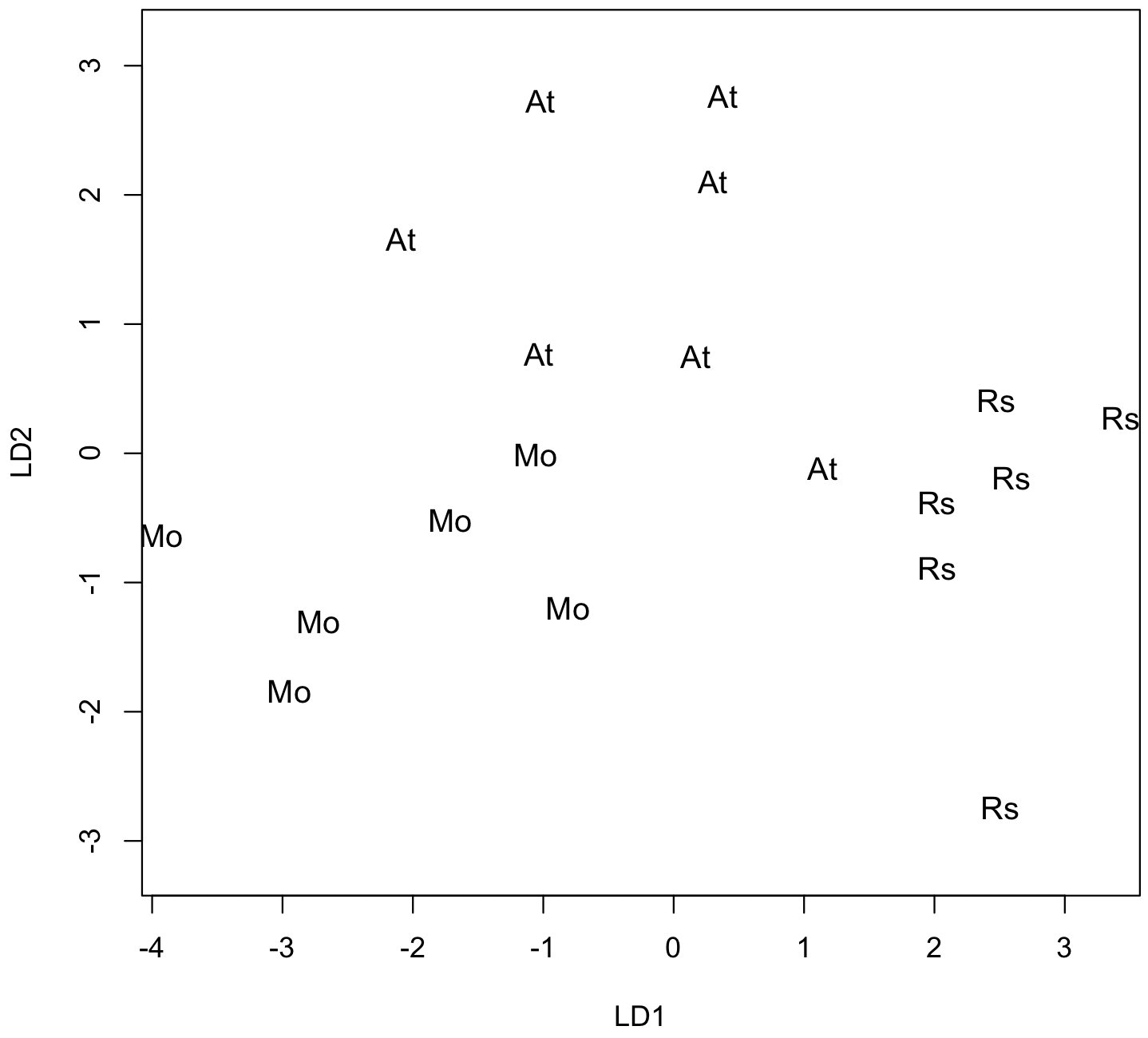
In this plot, the regions of the three groups largely do not overlap, although one case of group 1 lies close to group 2. This is a pattern that reflects successful discrimination of the groups.
A second type of plot shows how the data plot along a particular discriminant function:
plot(LDA, dimen=1, type="both")
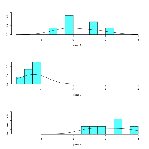
Again, note the good separation of the groups along discriminant function 1, particularly so for group 2.
Understanding the LDA functions
The scaling value of the lda object gives the loadings (also called the slopes, coefficients, or weights) of each variable on each discriminant function.
round(LDA$scaling, 2)
This produces a table with the columns corresponding to the discriminant functions and the rows corresponding to the variables used in the LDA. Each discriminant function should be scanned for the largest loadings, positive or negative, indicating the variables that contribute most to that discriminant function.
LD1 LD2 HCO3 1.68 0.64 SO4 -0.08 0.03 Cl -22.28 -0.31 Ca 1.27 2.54 Mg 1.89 -2.89 Na 20.87 1.29
In this case, Na has a strong positive loading, and Cl has a strong negative loading on the first discriminant function, and these are much larger than the loadings of the other variables, indicating that the Na:Cl ratio dominates LD1. Ca has a strong positive loading on the second discriminant function, with Mg having a strong negative loading, indicating that LD2 is dominated by the Ca:Mg ratio, although the relatively large loadings of Na and HCO3 indicate that they also influence the second discriminant function.
These interpretations can be confirmed by comparison with the log-transformed data used in the LDA.
cor(predictions$x[ , 1], brineLog$Na / brineLog$Cl) cor(predictions$x[ , 2], brineLog$Ca / brineLog$Mg)
As expected, these indicate a strong correlation of Na:Cl with LDA 1 (r=0.85) and a positive but weaker correlation of Ca:Mg with LDA 2 (r=0.69).
Evaluating the LDA
The effectiveness of LDA in classifying the groups must be evaluated, and this is done by comparing the assignments made by predict() to the actual group assignments. The table() function is most useful for this. By convention, it is called with the known assignments as the first argument and the fitted assignments as the second argument:
acc <- table(brineLog$GROUP, predictions$class) acc
The rows in the output correspond to the groups specified in the original data, and the columns correspond to the group assignments predicted by the LDA. In a perfect classification, all cases would fall on the diagonal, meaning the off-diagonal values would all be zero. This would indicate that the LDA discriminated all samples that belong to group 1 as belonging to group 1, and so on. The form of this table can give you considerable insight into which groups are reliably discriminated. It can also show which groups are likely to be confused and which types of misclassification are more common than others.
The following command calculates the overall predictive accuracy, that is, the proportion of cases that lie along the diagonal:
sum(diag(acc)) / sum(acc)
Here the predictive accuracy is almost 95%, quite a success. This approach measures what is called the resubstitution error, how well the samples are classified when all the samples are used to develop the discriminant function. The problem with this approach is that each case is used not only to build the discriminant function but also to test it.
A second and better approach for evaluating an LDA is leave-one-out cross-validation (also called jackknifed validation), which excludes one observation, formulates a discriminant function using the remaining data, and uses that function to classify the excluded observation. The advantage is that the classification is not based on the excluded sample. This cross-validation is done automatically for each sample in the data set. To do this, add CV=TRUE (think Cross-Validation) to the lda() call:
jackknife <- lda(GROUP ~ HCO3 + SO4 + Cl + Ca + Mg + Na, data=brineLog, CV=TRUE)
The success of the discrimination is measured with the same type of table as used in the resubstitution analysis:
accJack <- table(brineLog$GROUP, jackknife$class) accJack sum(diag(accJack)) / sum(accJack)
In this data set, the jackknifed validation is considerably less accurate (only 79%, compared with 95% for resubstitution), reflecting that resubstitution error always overestimates the performance of an LDA.
Predicting unknowns
One of the great uses of LDA is to develop a classification from a set of knowns (cases in which the group membership is known, as shown above) and use it to predict the groups of unknowns, cases in which the group membership is not known.
To do this, you will need a data frame set up as for your knowns, with the same column names but with no column for group membership. With this, use the predict() function and the LDA model to predict the classification of the unknown samples.
unknowns <- read.table("brineUnknowns.txt", header=TRUE, sep=",") unknownsLog <- log(unknowns+1) predict(LDA, unknownsLog)$class
This will return a vector showing the group to which each unknown case fits best.
What to report
When running a LDA, you should report the following:
- A table of the loadings that highlights the variables most important to each discriminant function.
- The proportion of the among-group variation that is explained by each discriminant function, as reported by the proportion of the trace.
- A plot of the LDA classification that plots the data coded by their actual groups against the LDA function(s). If there are more than two LDA functions, more than one plot will be necessary to show all of the functions.
- The jackknifed accuracy, or possibly also the resubstitution accuracy. Make clear which is reported.
References
Maindonald, J., and J. Braun, 2003. Data Analysis and Graphics Using R. Cambridge: Cambridge, 362 p.
Davis, J.C., 2002. Statistics and Data Analysis in Geology, Third Edition. Wiley: New York, 638 p.
