Generalized Linear Models
Linear models, as produced by the lm() function, make several critical assumptions: normally distributed errors, constant variance, and no trends in residuals relative to fitted values. When these assumptions will be violated, you must use a different modeling procedure, such as Generalized Linear Models. Generalized linear models are implemented in R with the glm() function, which has the same model syntax as lm() and aov(). Generalized linear models use likelihood methods, so they fundamentally differ in their approach from least-squares regression.
Generalized linear models have three important components: the error structure, the linear predictor, and the link function.
The error structure describes how the errors are distributed. Count data, represented as integers with a minimum value of zero, have Poisson-distributed errors. Proportions, which range from zero to one, have binomial-distributed errors. Data with a constant coefficient of variation, where standard deviation is a multiple of the mean, have gamma-distributed errors. Survival data, also called time-to-death data, have errors that follow an exponential distribution. Any time that you deal with such counts, proportions, or survival data, you should use a generalized linear model rather than a simple least-squares regression.
The linear predictor is the sum of the parameters (slopes), each multiplied by the values of the explanatory variables. It is formed by the right side of the linear model formula.
The link function is a function that relates the mean value of y to the linear predictor and may be the most confusing aspect of a generalized linear model. Every error structure has an associated link function. The normal distribution has a link function called the identity function, which means that the y-value equals the linear predictor. In other words, nothing must be done to relate the y-value to the linear predictor. In glm(), the family argument specifies the error distribution and link function. For example, to set a Gaussian error model and an identity link function, just set the family to be Gaussian:
glm(y ~ x, family=gaussian)
This will produce the same results as if you had called lm(), although glm() calculates the regression coefficient with likelihood methods, not by minimizing the sum of squares as lm() does.
Here are the most common settings for family in glm() and their associated link functions. Notice that only Gamma is capitalized.
- family=binomial (link: logit)
- family=gaussian (link: identity)
- family=Gamma (link: inverse)
- family=poisson (link: log)
Likelihood, deviance, and AIC
Because generalized linear models are based on likelihood, their output differs somewhat from common non-likelihood methods like t-tests, F-tests, ANOVA, correlation, and least-squares regression. In particular, generalized linear models report null deviance, residual deviance, and AIC (the Akaike Information Criterion). Deviance equals two times the log-likelihood ratio of a model compared with a saturated model, that is, a model that fits every data point perfectly. Smaller values indicate a good model fit. Null deviance compares a single-parameter model (the mean of the response variable) to the saturated model. Usually such a fit will be quite poor, causing null deviance to be large. Residual deviance compares the fit of the generalized linear model to the saturated model. If the generalized linear model fits well, residual deviance will be markedly smaller than the null deviance.
Whether this drop in deviance is statistically significant can be evaluated similarly to how an F-test is used to assess the statistical significance of a least-squares regression. The p-value is calculated using the difference in the null and residual deviances and the difference in null and residual degrees of freedom using a chi-squared distribution.
The output of a generalized linear model also reports the AIC. This value is of little use by itself, but it could be used to compare different models fitted to the same data, especially when they differ in their number of parameters. The model with the lowest AIC would be the preferred model.
Explained variance
The glm() function does not produce coefficients of determination (R2), but it can be calculated easily from the model (see stats.stackexchange). Similar to how the coefficient of determination is generally defined as 1 minus the sum of squares of residuals divided by the total sum of squares, the deviance-based approach uses 1 minus the model deviance divided by the null deviance. The r2glm() function will calculate the coefficient of determination; its only argument is the model fitted by glm().
r2glm <- function(model) { rsq <- 1 - model$deviance / model$null.deviance return(rsq) }
Count data
Count data have several important properties. First, count data have a minimum value of zero and are therefore said to be bounded below. Count data are integers, which affects their error distribution; in other words, their errors are discrete, not continuous. Last, count data follow a Poisson distribution in which variance is not constant and increases with the mean.
A generalized linear model for count data requires the Poisson family and would therefore be written as
glm(y~x, family=poisson)
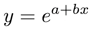
This model is equivalent to the equation

which can be rewritten as

where y is counts and x is some independent variable thought to control the counts. a and b are the regression coefficients to be fitted to the data.
To fit a generalized linear model to count data, put the counts in one vector and the explanatory vector in another. For this example, we will use the flora.csv data set, which contains two vectors of interest, elevation and maple. Our goal is to model maple tree abundance as a function of elevation. As always, we plot the data before fitting a model. We will use glm() to fit the model using a Poisson family.
flora <- read.table("flora.csv", header=TRUE, sep=",") attach(flora) plot(elevation, maple, las=1, pch=16, col="green") model <- glm(maple~elevation, family=poisson)
View the results of the model with summary(), coef() to extract the fitted coefficients a and b, and confint() to generate the confidence intervals on those coefficients.
summary(model) coef(model) confint(model)
To add the fitted regression curve to the plot, use the predict() function to generate the points along the curve at specified x values. The predict() function can be used with all types of regression to display the regression curve on a plot.
elevationPoints <- seq(min(elevation), max(elevation), by=0.01) fittedValues <- predict(model, list(elevation=elevationPoints), type="response") lines(elevationPoints, fittedValues, lwd=3, col="blue")
Because glm() models are based on likelihood methods, the output of summary()differs from lm() models.
Call: glm(formula = maple ~ elevation, family = poisson) Deviance Residuals: Min 1Q Median 3Q Max -2.2948 -1.1941 -0.5495 1.0081 2.1554 Coefficients: Estimate Std. Error z value Pr(>|z|) (Intercept) 7.58051 0.50482 15.02 <2e-16 *** elevation -0.28749 0.02794 -10.29 <2e-16 *** --- Signif. codes: 0 *** 0.001 ** 0.01 * 0.05 . 0.1 1 (Dispersion parameter for poisson family taken to be 1) Null deviance: 143.656 on 19 degrees of freedom Residual deviance: 35.216 on 18 degrees of freedom AIC: 105.5 Number of Fisher Scoring iterations: 5
Deviance Residuals should be checked for symmetry: the median value should be close to zero, and the 1Q and 3Q values should be roughly equidistant from the median. Max and Min should also be roughly equidistant from the median, but as endpoints, they are likely to deviate more than 1Q and 3Q.
The table also provides z-scores and p-values based on the z-scores to test whether the coefficients are significantly different from zero
The markedly lower residual deviance compared with the null deviance indicates a good model fit. The corresponding p-value is calculated using the difference in the null and residual deviances and the difference in the null and residual degrees of freedom using a chi-square distribution. For this model, the p-value could be calculated as follows:
pchisq(model$null.deviance - model$deviance, model$df.null - model$df.residual, lower.tail=FALSE)
Because we are only interested in a drop in deviance, we want to focus on the upper tail of the distribution and therefore set lower.tail=FALSE.
Proportion and binary data
Proportion data have three important properties. Values are constrained to lie between 0 and 1, inclusive, and are therefore said to be strictly bounded. The errors are non-normally distributed and follow a binomial distribution. Finally, variance is not constant, reaching a minimum when the proportions are near zero and one and reaching a maximum when the proportion is 0.5.
Proportion and binary data require the binomial family, which uses a logit link function. The logit function equals log(p/(1-p)), also called the log-odds, where p is the proportion. The model for proportion or binary data is stated as
glm(p~x, family=binomial)
This model specifies the relationship

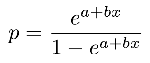
which can be rewritten in terms of p as:

where p is the proportion and x is the independent variable thought to control the proportion. a and b are the model coefficients to be fitted.
Example 1: proportions
The first example will be for proportional data, where we will model the proportional abundance of maple trees in forest communities as a function of elevation. The data come from the flora.csv data set, which contains three columns: maple, otherTrees, and elevation.
flora <- read.table("flora.csv", header=TRUE, sep=",") attach(flora)
To plot the data, we will calculate the proportion of the community represented by this species as a function of elevation.
proportion <- maple/(otherTrees+maple) plot(elevation, proportion, las=1, pch=16)
To fit the model and preserve information on sample size, we need to combine the abundances of maples and the other trees into a single matrix (abundances), using the cbind() function (think “column bind”). The model is fitted with glm(), specifying the community data as a function of elevation, using the binomial family because this is proportional data.
abundances <- cbind(maple, otherTrees) model <- glm(abundances~elevation, family=binomial)
As usual, view the results of the model with summary(), use coef() to extract the fitted coefficients a and b, and use confint() to generate the confidence intervals.
summary(model) coef(model) confint(model)
To added the fitted relationship to the plot, create a vector of elevation values along which the fitted relationship will be calculated. Use predict() to generate those proportions, then use lines() to add this curve to the plot with the data.
elevationValues <- seq(min(elevation), max(elevation), by=0.01) fittedValues <- predict(model, list(elevation=elevationValues), type="response") lines(elevationValues, fittedValues, lwd=3, col="forestgreen")
Alternatively, you could put the proportions in a vector (done above), and the sample sizes in a second vector. As before, glm() is used to fit the model, specifying a binomial family and setting the weight to equal the sample size. This will produce the same model as the first approach.
sampleSize <- maple + otherTrees model <- glm(proportion~elevation, family=binomial, weights=sampleSize) detach()
Example 2: binary data
This same model can also be used for binary data, such as the occurrence of a species along a habitat transect, which are recorded as 1’s (present) and 0’s (absent). For this we will use the floraPA.csv data set, which contains the presence (1) or absence (0) of pine trees (pine) with temperature. The first step is to plot the data.
floraPA <- read.table("floraPA.csv", header=TRUE, sep=",") attach(floraPA) plot(temperature, pine, las=1, pch=16)
The model is fitted with glm(), setting the family argument to binomial.
model <- glm(pine ~ temperature, family=binomial)
Model results, coefficients, and confidence intervals are extracted in the usual way.
summary(model) coef(model) confint(model)
The fitted relationship is added to the plot following the same approach.
temperatureValues <- seq(min(temperature), max(temperature), by=0.01) fittedValues <- predict(model, list(temperature=temperatureValues), type="response") lines(temperatureValues, fittedValues, lwd=3, col="forestgreen")
Survival data
Survival data, also called time-to-death and time-to-failure data, have nearly always non-constant variance. Where these data have errors that follow a gamma distribution, variance is proportional to the square of the mean, which causes variance to increase more rapidly than the mean. Gamma errors require a reciprocal link function (1/y), and their model is written as:
glm(y~x, family=Gamma)
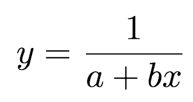
This model specifies the relationship

or, alternatively

where y is the survival time (or time to death or failure), x is the predictor variable, and a and b are the coefficients to be fitted.
Survival data can be fitted with the time-to-death data in one vector and the explanatory vectors in another. The function calls and plotting are similar to those above, but set the family argument to Gamma (remember to capitalize it as opposed to all the other families, which are not capitalized).
References
Dalgaard, P. 2002. Introductory statistics with R. Springer-Verlag, New York.
Sokal, R. R., and F. J. Rohlf. 1995. Biometry. W.H. Freeman and Company, New York.
Verzani, J. 2005. Using R for introductory statistics. Chapman & Hall / CRC Press, Boca Raton, Florida.
