Likelihood Methods
Most classical statistics focus on testing null hypotheses, often the so-called zero-null hypothesis of no difference or relationship. Not only is the zero-null hypothesis rarely of interest in itself, but it is usually known to be false even before data collection begins. Rather than test a single uninteresting hypothesis, it is usually far more useful to test a range of hypotheses and find which hypothesis is most supported by the data. This is known as model selection, and likelihood methods are a common model selection method. The measure of support for a model is called likelihood.
Likelihood and probability sound like synonyms but are not, even though the distinction can seem subtle. Probability allows us to predict outcomes (data, statistics) based on a hypothesis, whereas likelihood measures the support our data offer a specific model. Likelihood will also allow us to estimate the parameters of models. In other words, we speak of the probability of data (given a model or hypothesis), or the likelihood of a model (given some data).
Likelihood is proportional to the probability of observing the data given the hypothesis; this is similar to a p-value but does not include the tail of the distribution. Because we are generally interested in relative likelihood, that is, the support for one hypothesis compared to another, we can ignore the proportionality constant linking likelihood to probability.
Probability and likelihood have another important distinction. In probability, the sum of the probabilities of all outcomes must equal 100% for any given hypothesis. This is because there are a finite number of possible outcomes for any hypothesis or model, and therefore, their probabilities must sum to 100%. For likelihood, there are potentially an infinite number of models that might explain the data. As a result, the sum of all likelihoods generally does not equal 100%, and it may not even be a finite number.
We can plot likelihood as a function of a parameter, every value of which represents a particular hypothesis. For example, every possible slope is a hypothesis for the relationship between two variables. The slope that has the highest likelihood is the best-fit parameter value, that is, it is the hypothesis most supported by the data. The parameter that makes the likelihood as large as possible is called the maximum likelihood estimate (MLE).
The shape of a likelihood curve is important. A more steeply dipping curve suggests that the parameter estimate is better constrained than a curve that is nearly flat. A relatively flat likelihood curve suggests that many hypotheses are almost equally likely.
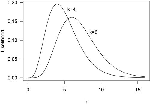
An example helps to understand likelihood. Suppose we have measured the number of events in a given amount of time, k, a statistic based on our sample. We could fit likelihood curves for the average number of events per unit of time (r, short for rate), which is a parameter of the population. When four events are measured in an interval of time (k=4), the likelihood curve for the modeled rate of events unsurprisingly reaches a maximum at r=4, making that the best parameter estimate for the average number of events per time. Likewise, if we observed 6 events, the likelihood function for k=6 reaches a maximum at r=6.
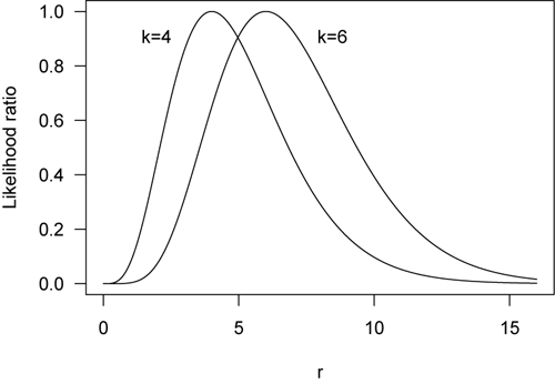
Likelihood curves are often scaled by their maximum value, producing what is called the likelihood ratio. The maximum likelihood estimate on a likelihood-ratio curve therefore has a value of 1.0. Here are the previous two curves now plotted as likelihood ratios.
Because likelihoods may be very small numbers, the natural (base-e) logarithm of likelihood is usually plotted. When the log of likelihood is plotted as a function of the parameter, it is called the support function. On a support function curve (not shown), the highest log-likelihood value corresponds to the best parameter estimate.
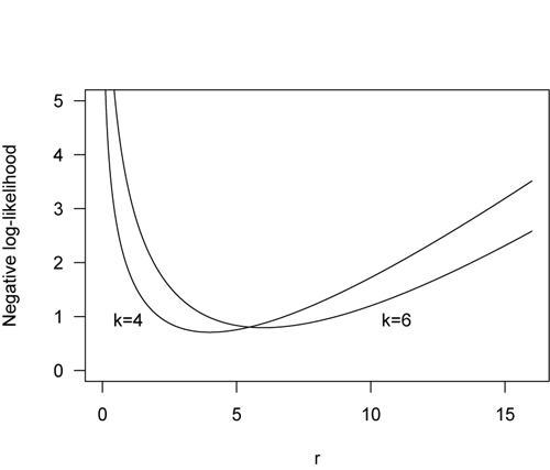
In traditional statistics, we often try to minimize a sum of squares. For example, we do this in a least-squares regression, where the lowest sum of squares of the residuals corresponds to the least error. By plotting the negative log-likelihood, we follow the same convention: we seek the minimum of the negative log-likelihood (shown below). One advantage to using negative log likelihoods is that we might have multiple observations and want to find their joint probability. This would normally done by multiplying their individual probabilities, but if we use log-likelihood, we can simply add those probabilities.
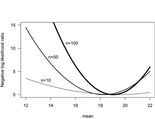
Negative log-likelihood curves become steeper and more compressed as sample size increases, indicating greater certainty in our parameter estimate. The plot below shows the likelihood curves for four estimates of a mean, as a function of sample size. Note that the curve for n=100 is narrow, indicating less uncertainty in the estimate of mean than for n=10, which has broad and flat likelihood curve.
An Example
We will not dwell on the calculation of likelihood nor have any homework on this. If you are interested in likelihood solutions, you will consult a reference for the appropriate formulas.
Even so, we an demonstrate performing a linear regression through a likelihood function. First, we start with bivariate data.
x <- c(21.27, 17.31, 11.83, 16.73, 19.82, 18.25, 16.29, 16.17, 13.84, 15.12) y <- c(87.72, 74.01, 57.22, 67.07, 78.87, 78.87, 68.93, 61.22, 55.40, 59.07)
We need to specify a range of slopes over which we will search for the regression that best fits the data. If the likelihood curve does not reach a maximum over this range, we will need to broaden our search of possible slopes. We will search for possible slopes the interval from 2 to 6 to the nearest 0.01. We will store these slopes as matrix, not as a vector. If we want greater precision in our slope estimate, we would choose a value smaller than 0.01.
slopes <- matrix(seq(from=2, to=6, by=0.01), ncol=1)
Next, we calculate the likelihood of each slope in our range, storing them in lik. Although this could be done with a loop, it’s better to avoid loops in R, which can often be done with apply() or one of its relatives. The apply() function takes the vector of slopes (slopes), and for each row (slope; MARGIN=1), performs a set of calculations on that slope (b1). Here, it calculates the product of the probabilities of the deviations from a line with a given slope, assuming that the deviations are normally distributed with a mean of zero and a standard deviation of 1. Note that this also assumes that the y-intercept is zero.
lik <- apply(slopes, MARGIN=1, function(b1) { deviations <- y - b1*x prod(dnorm(deviations, mean=0, sd=1)) })
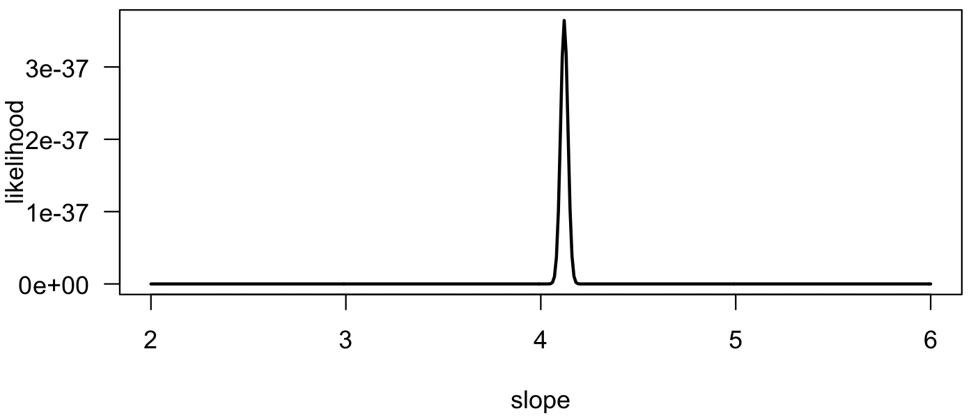
We can plot the likelihood curve and see that it reaches a well-defined maximum near 4.1, which is our maximum likelihood estimate for the slope.
plot(slopes, lik, type="l", las=1, xlab="slope", ylab="likelihood", lwd=2)
We can compare the maximum likelihood estimate with the estimate from a least-squares approach and see that they have similar values.
slopes[which(lik==max(lik))] lm(y~x)
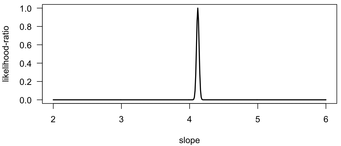
We can also plot the likelihood ratio. The shape of the curve is unchanged, but the y-axis is rescaled to go from zero to one, with the maximum likelihood estimate at 1.
likRatio <- lik/max(lik) plot(slopes, likRatio, type="l", las=1, xlab="slope", ylab="likelihood-ratio", lwd=2)
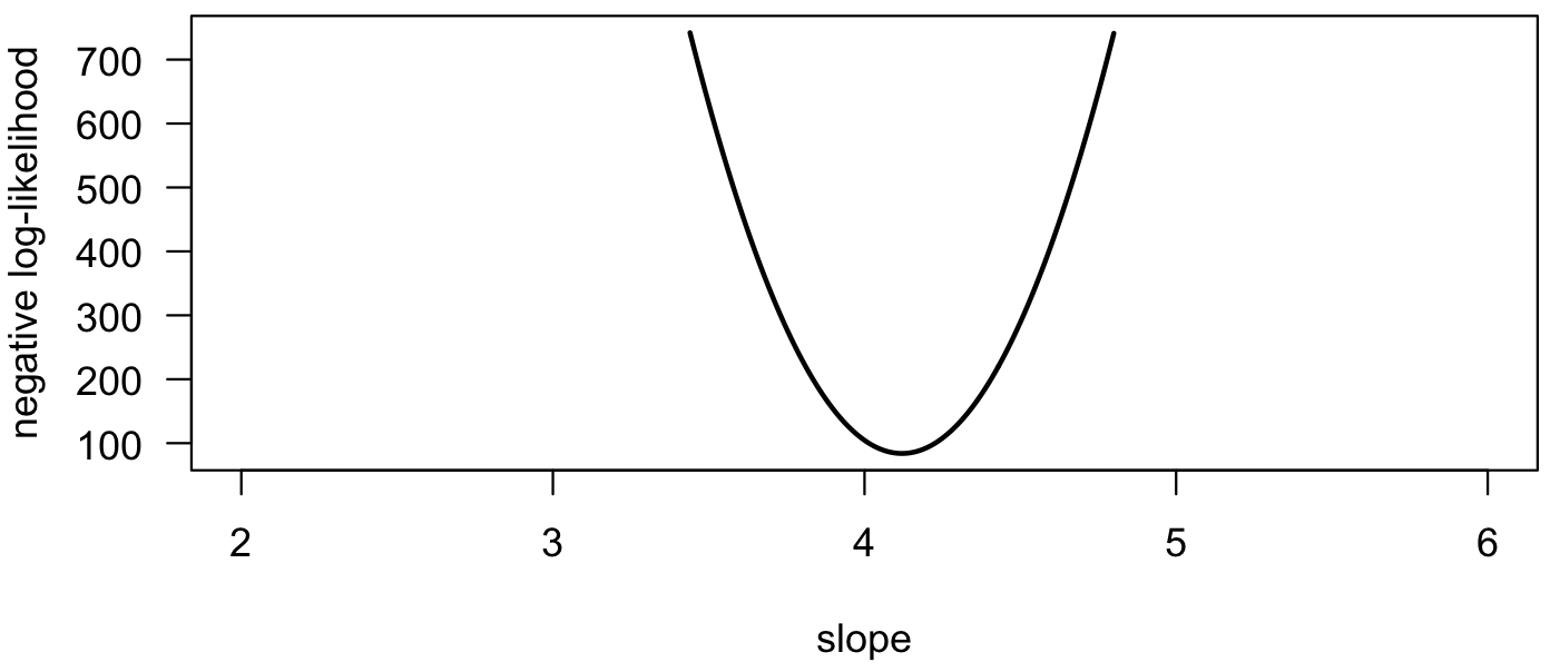
We can also plot the negative log-likelihood. Notice that the maximum likelihood estimate is at the minimum on this curve. Using the logarithm causes the curve to be less peaked than on previous plots.
negLogLik <- -log(lik) plot(slopes, negLogLik, type="l", las=1, xlab="slope", ylab="negative log-likelihood", lwd=2)
Rather than find the best-fit model from a graph, we can also optimize the function to find the maximum likelihood estimate. First, we define a function to be minimized. For this example, the deviations to the line will be minimized. For simplicity, it is assumed that the y-intercept is zero. NLL is the negative log-likelihood
slopeNLL <- function(slope, x, y) { deviations <- y - slope*x NLL <- -sum(dnorm(deviations, mean=0, sd=1, log=TRUE)) NLL }
Next, the minimum of this function is sought because it corresponds to the fit with the smallest residuals. We provide optim() a starting point for the slope near what we suspect the minimum is; here we set it to 7, and we could also have chosen any other nearby value.
optSlope <- optim(fn=slopeNLL, par=c(slope=7), x=x, y=y, method="BFGS") optSlope
In the output, optSlope$par gives the estimate for slope, and optSlope$value gives the negative log-likelihood. This is essentially the same as finding the maximum, as shown above, where the likelihood slope was compared to a least-squares slope.
Confidence Intervals
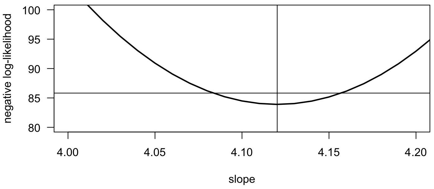
Likelihood approaches not only generate parameter fits and allow you to select the most appropriate model, they can also generate confidence intervals on parameters. These are generally method-specific, and there are several ways that these can be calculated. The profile likelihood confidence interval is easiest to calculate for a one-parameter model. For it, the 95% confidence interval corresponds to the range of parameters for which the log-likelihood lies within 1.92 of the maximum log-likelihood value. On a plot of negative log-likelihood, a horizontal line drawn 1.92 units above the minimum value will intersect the negative log-likelihood function at the upper and lower confidence limits. The value of 1.92 is one-half the 95% critical value for a χ2 (pronounced Chi-squared) distribution with one degree of freedom. This can be calculated in R as qchisq(p=0.95, df=1)/2.
Zooming in on our example, we can use the results of the optimization to show the estimate and the confidence interval:
plot(slopes, negLogLik, type="l", las=1, xlab="slope", ylab="negative log-likelihood", lwd=2, xlim=c(4.0, 4.2), ylim=c(80, 100)) abline(v=optSlope$par) abline(h=optSlope$value + 1.92)
Given the growing emphasis on parameter estimation and placing uncertainty estimates on those parameters, likelihood methods are increasingly popular. Gains in computing processing speeds make likelihood methods increasingly accessible.
Model Selection
One of the great advantages of likelihood approaches is that they allow you to select the best-fitting model from a group of models that may differ in the number of parameters. When we compare models with the same number of parameters, the best model will be the one with the maximum likelihood or equivalently, the smallest (most negative) negative log-likelihood. For example, our strategy in fitting a regression with two parameters would be to search the entire space of slope-intercept combinations and find the pair of parameters with the maximum likelihood. As you can imagine, this can be computationally expensive for complicated models.
When competing models differ in the number of parameters, we cannot use this simple approach. When one model is nested within another, such as a linear regression (with parameters for slope and intercept) versus a quadratic regression (with parameters for curvature, slope, and intercept), we can use the Likelihood Ratio Test and calculate the likelihood ratio (R):
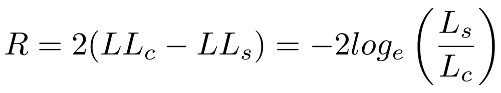
where LLc is the log-likelihood of the more complex model and LLs is the log-likelihood of the simpler model (Lc and Ls are the likelihoods). R follows a χ2 (chi-squared) distribution, with the degrees of freedom equal to the difference in the number of parameters of the two models. A p-value can be obtained from pchisq().
When models are not nested but differ in the number of parameters, we cannot use a likelihood ratio test. Instead, an information criterion is used, which is based on the negative log-likelihood plus a penalty for the number of parameters. Because models with more parameters generally have a better fit, the penalty ensures that a more complicated model must improve substantially over a simple one to be considered the best one. The model with the lowest information criterion is the best model. The Akaike Information Criterion (AIC) is the most common information criterion and is calculated as:

where Li is the log-likelihood, and Ki is the number of parameters in model i. The Akaike Information Criterion finds the best model with the fewest parameters. The Bayesian Information Criterion (BIC) is less commonly used and has a penalty parameter of K*log(n), where n is the sample size. BIC is more conservative than AIC.
This example from Gene Hunt’s work shows a typical table in which likelihood and information criteria are used to evaluate evolutionary models of varying complexity (Hunt 2008).

These models vary in their number of parameters (K), making them difficult to compare. If they had the same number of parameters, the best model would be the one with the highest log-likelihood (Log(L)): model 7, or sampled punctuation (directional evolution transition). Because more complex models are more likely to offer a better fit, one must use an information criterion. Here, Gene uses AICc, and the best model is the one with the lowest (most negative) value: model 6, or sampled punctuation (unbiased random walk transition).
Akaike weights (w) can also be used to determine which model or models have the most support. First, calculate the relative likelihood of each model i, or exp[-0.5 * (AICi-AICmin)], where AICmin is the smallest AIC value among all the models. The weight for each model is the relative likelihood for that model divided by the sum of these relative likelihoods. The sum of the weights will equal 1. The model with the largest weight is the preferred model. This will always be the model with the lowest AIC value (model 6).
Supplemental likelihood code
This is the code for generating the four plots illustrating likelihood at the beginning of these notes.
# Poisson demonstration rate <- seq(0, 16, 0.01) k4 <- 4 k4Like <- c() k6 <- 6 k6Like <- c() for (i in 1:length(rate)) { k4Like[i] <- dpois(k4, rate[i]) k6Like[i] <- dpois(k6, rate[i]) } # likelihood curves plot(rate, k4Like, type="l", xlab="r", ylab="Likelihood", las=1) points(rate, k6Like, type="l") text(5, 0.18, "k=4", pos=4) text(8, 0.12, "k=6", pos=4) # Likelihood ratio curves k4LikeRatio <- k4Like/max(k4Like) k6LikeRatio <- k6Like/max(k6Like) plot(rate, k4LikeRatio, type="l", xlab="r", ylab="Likelihood ratio", las=1) points(rate, k6LikeRatio, type="l") text(1, 0.9, "k=4", pos=4) text(7.5, 0.9, "k=6", pos=4) # Negative log-likelihood curves k4NegLogLike <- -log10(k4Like) k6NegLogLike <- -log10(k6Like) plot(rate, k4NegLogLike, type="l", xlab="r", ylab="Negative log-likelihood", las=1, ylim=c(0,5)) points(rate, k6NegLogLike, type="l") text(0, 0.9, "k=4", pos=4) text(10, 0.9, "k=6", pos=4) ####### Effect of sample size ######## # Generate data and sub samples data <- rnorm(100, mean=17.3, sd=8.2) n <- 50 sub50 <- sample(data, n) n <- 10 sub10 <- sample(data, n) # Negative log-likelihood ratio for entire data means <- seq(12, 22, 0.01) NLL <- rep.int(0, times=length(means)) for (i in 1:length(means)) { deviations <- data-means[i] deviations.standardized <- deviations/sd(deviations) NLL[i] <- sum(-log(dnorm(deviations.standardized, mean=0, sd=1))) } NLL <- NLL-min(NLL) plot(means, NLL, type="l", las=1, xlab="mean", ylab="Negative log-likelihood ratio", lwd=4, ylim=c(0, 15)) # Negative log-likelihood ratio for first subset for (i in 1:length(means)) { deviations <- sub50-means[i] deviations.standardized <- deviations/sd(deviations) NLL[i] <- sum(-log(dnorm(deviations.standardized, mean=0, sd=1))) } NLL <- NLL-min(NLL) points(means, NLL, type="l", las=1, xlab="slope", ylab="Negative log-likelihood", lwd=2) # Negative log-likelihood ratio for second subset for (i in 1:length(means)) { deviations <- sub10-means[i] deviations.standardized <- deviations/sd(deviations) NLL[i] <- sum(-log(dnorm(deviations.standardized, mean=0, sd=1))) } NLL <- NLL-min(NLL) points(means, NLL, type="l", las=1, xlab="slope", ylab="Negative log-likelihood", lwd=1) text(15, 11, pos=4, "n=100") text(13.6, 8, pos=4, "n=50") text(13, 3, pos=4, "n=10")
References
Bolker, B.M., 2008. Ecological models and data in R. Princeton University Press, 396 p.
Hilborn, R., and M. Mangel, 1997. The ecological detective: Confronting models with data. Monographs in Population Biology 28, Princeton University Press, 315 p.
Hunt, G., 2008. Gradual or pulsed evolution : When should punctuational explanations be preferred? Paleobiology 34:360–377.
