Testing central tendency
One of the most common tasks in data analysis is evaluating central tendency, the expected value in a distribution. Central tendency is most commonly measured with the mean or the median. We will learn how to estimate central tendency and its uncertainty with confidence intervals, and we will learn how to test hypotheses about central tendency.
Arithmetic mean
The arithmetic mean is the sum of observations divided by sample size (n). The statistic mean is symbolized by an X with a bar over the top (x̄), and the parameter mean is symbolized by the Greek letter μ (mu).
The sample mean is an unbiased estimator of the population mean; in other words, the sample mean is equally likely to be larger than or smaller than the population mean. The sample mean is also an efficient statistic compared to the sample median, meaning that the sample mean is more likely to lie closer to the population mean than the sample median is to the population median. These are both good things: we want unbiased and efficient statistics.
To make statistical inferences, we must know how a sample statistic is distributed when sampling from a population with given parameters (the null hypothesis). In this case, we need to understand how the sample mean is distributed, given by the central limit theorem:
The means of samples drawn from a population of any distribution will be approximately normally distributed, and this approximation gets better as the sample size increases.
In other words, as long as the sample size is sufficiently large, sample means will be normally distributed. How large constitutes “sufficient’ depends on the parent distribution. If the the parent distribution is normally distributed, the sample means of even quite small samples (n=10) will closely approximate a normal distribution. However, for markedly non-normal parent distributions, sample size might need to be at least 100 or more for sample means to be approximately normally distributed.
A distribution of sample means has two important characteristics. First, the expected value of a sample mean is the population mean, that is the average value of sample means is equal to the population mean. This lets us use the sample mean as an estimate of the population mean.
Second, the standard deviation of the distribution of sample means equals the standard deviation of the parent population (σ) divided by the square root of the sample size (n). This quantity is called the standard error of the mean:
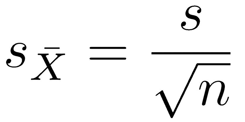
A standard error describes the standard deviation of a sample statistic; it is called a standard error to avoid confusing it with the standard deviation of the data. Because the standard error of the mean is calculated by dividing the standard deviation of the data by the square root of n, increasing the sample size quickly shrinks the standard error of the mean. In other words, increasing the sample size reduces the uncertainty in the mean. As we have seen before and will continue to see, increasing sample size brings many benefits, so you should always increase sample size as large as time and money allow.
The central limit theorem in action
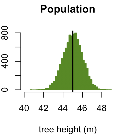
We can simulate how the central limit theorem works. For the first simulation, we will assume that the variable we are measuring is normally distributed; in other words, we would say that the parent distribution is normal. To help make matters more concrete, we will imagine that we are measuring the heights of trees that have a mean height of 45 m.
dev.new(width=3, height=3) trees <- rnorm(10000, mean=45) lowerLimit <- floor(range(trees)[1]) upperLimit <- ceiling(range(trees)[2]) popRange <- c(lowerLimit, upperLimit) popBreaks <- seq(lowerLimit, upperLimit, by=0.1) hist(trees, breaks=popBreaks, ylab="", xlab="tree height (m)", main="Population", col="chartreuse4", border="chartreuse4", xlim=popRange, las=1) abline(v=mean(trees), col="black", lwd=2)
This first plot shows the distribution of tree heights in this forest. The vertical black line shows the mean height of 45 m. This is the mean of the population, but the mean of the population is generally unknown (unlike a simulation), so we want to estimate it based on a sample.
Next, imagine selecting a sample of a certain size from this population of trees, then calculating the mean of the trees in that sample. If you did this multiple times, you would get a somewhat different value every time. Although we would rarely collect a sample multiple times in real life (there’s not enough time or money), we can simulate this process of sampling and measuring the mean many times (10000). This will produce a distribution of sample means for that sample size. We will do this for four sample sizes, ranging from n=5 (top) to n=50 (bottom).
dev.new(width=3, height=8) par(mfrow=c(4,1)) trials <- 10000 sampleSize <- c(5, 10, 20, 50) for (j in 1:length(sampleSize)) { sampleMean <- replicate(n=trials, mean(sample(trees, size=sampleSize[j]))) par(mar=c(4, 4, 4, 2) + 0.1) hist(sampleMean, ylab="", xlab="mean tree height (m)", xlim=popRange, main=paste("Sample Means, n=", sampleSize[j], sep=""), col="chartreuse2", border="chartreuse2", breaks=popBreaks, las=1) }
The plot below shows the four distributions of sample means, each corresponding to a different sample size. To help make comparisons, all four plots are at the same scale, the same as the one for the original data.
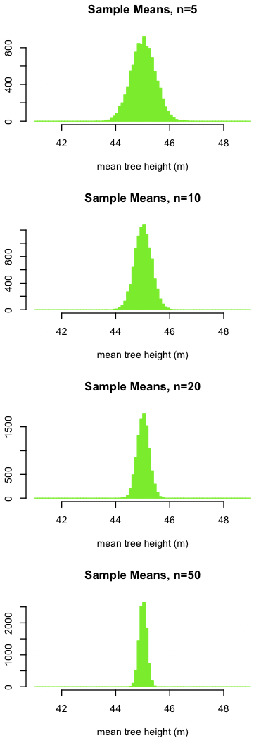
Notice three things:
- The sample means appear to be normally distributed.
- The mean of the sample means is the same as the mean of the parent population, about 45 m. In other words, the sample mean can be used to estimate the population mean.
- As the sample size increases, the variation in the sample means decreases. In other words, our estimate of the population mean gets better as the sample size grows because the uncertainty in the sample mean decreases.
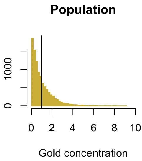
Perhaps it doesn’t seem surprising that the sample means are normally distributed, given that the parent distribution of tree heights is normal. This isn’t a fluke, though. We can show that by performing the same simulation, but one based on a markedly non-normal distribution. The exponential distribution is a good choice because it is as asymmetric as you can get, as it has no left tail whatsoever: the entire distribution is in the right tail.
In this case, we will pretend this is the concentration of gold that we measure in a prospective ore body; you would expect most samples to have little or no gold, and only a few to have a lot of gold, so a right-tailed distribution makes sense. What the data are (gold vs. tree height) doesn’t matter; the only important part is the shape of the distribution.
dev.new(width=3, height=3) gold <- rexp(10000) lowerLimit <- floor(range(gold)[1]) upperLimit <- ceiling(range(gold)[2]) popRange <- c(lowerLimit, upperLimit) popBreaks <- seq(lowerLimit, upperLimit, by=0.1) hist(gold, breaks=popBreaks, ylab="", xlab="gold concentration", main="Population", col="gold3", border="gold3", xlim=popRange, las=1) abline(v=mean(gold), col="black", lwd=2)
The plot below shows the distribution of gold concentration: most samples have very little gold, but some have quite a bit. The vertical black line shows that the mean gold concentration in the population is 1.0. Again, we want to know the population mean, but we cannot collect the whole population (not enough time or money, as always). Instead, we collect a sample and measure its mean. If we were to repeat this, collect another sample, and measure its mean, we would get a slightly different value every time. We will simulate doing this many times (10000) to see how the sample mean is distributed.
dev.new(width=3, height=8) par(mfrow=c(4,1)) trials <- 10000 sampleSize <- c(5, 10, 20, 50) for (j in 1:length(sampleSize)) { sampleMean <- replicate(n=trials, mean(sample(gold, size=sampleSize[j]))) par(mar=c(4, 4, 4, 2) + 0.1) hist(sampleMean, ylab="", xlab="mean gold concentration", xlim=popRange, main=paste("Sample Means, n=", sampleSize[j], sep=""), col="gold", border="gold", breaks=popBreaks, las=1) }
The four plots below show the distribution of sample means for four different sample sizes. All four plots and the one above for the population are at the same scale.
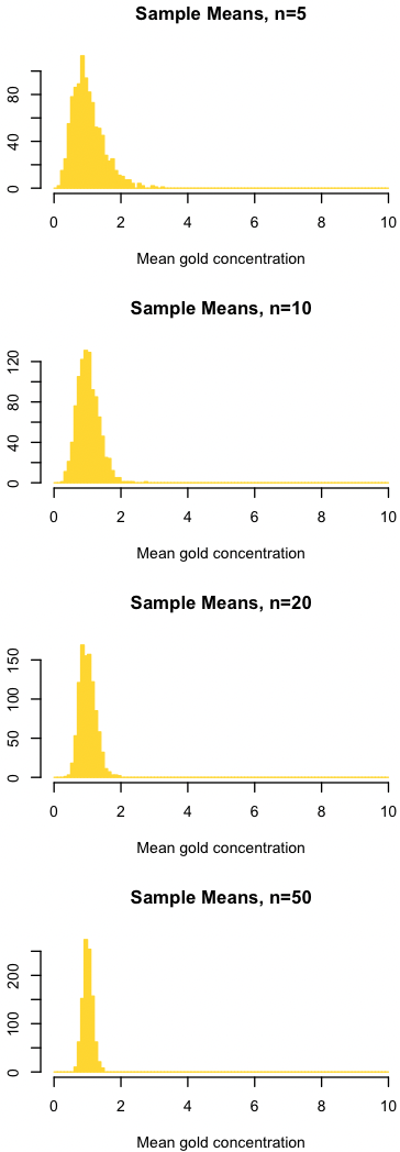
Like before, notice three things:
- As the sample size increases, the distribution of sample means better approximates a normal distribution. The approximation isn’t great at n=5, and the distribution of sample means is clearly right-tailed. As the sample size increases, the distribution becomes increasingly symmetrical, that is, it converges on a normal distribution.
- The mean of the sample means is the same as the mean of the parent population (1). Notice that the center of all four distributions is about the same as the population mean. In other words, the sample mean provides an estimate of the population mean.
- As the sample size increases, the variation in the sample means decreases. As before, our estimate of the population mean gets progressively better as our sample size increases.
The central limit theorem is useful because it shows that sample means will be approximately normally distributed, increasingly so at larger sample sizes, regardless of how the parent distribution is shaped. We can use this fact to calculate confidence intervals, p-values, and critical values for sample means. That said, we need to be attentive to the shape of the parent distribution: sample means will approximate a normal distribution at small sample sizes, but sample size may need to be rather large (>100) for this approximation to be true for non-normal parent distributions.
Parametric test: Student’s t-test
Our first hurdle is that there is an infinite number of normal distributions: imagine every possible combination of mean and standard deviation. Rather than create a test for every possible combination, we will perform a rescaling that will simplify this to many fewer distributions. We will make a rescaling called a t-statistic, which scales the width and center of the normal distribution. The t-statistic is calculated as:
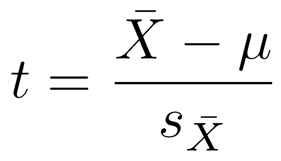
where X̄ is the sample mean, and μ is the null hypothesis about the population mean. The standard error of the sample mean (sX̄) is defined as the sample standard deviation divided by the square root of the sample size:
In R, the longhand way of calculating the t-statistic would work like this, but we will typically use even easier ways to calculate it:
t <- (mean(x) - nullHypothesis) / (sd(x) / sqrt(length(x)))
The t-statistic has an intuitive interpretation: it is the difference (distance) between our observed and hypothesized means, scaled by (divided by) the uncertainty in the sample mean (the standard error). Large positive values indicate that the observed mean is much larger than the null hypothesis; values near zero would indicate that the mean and the null hypothesis are essentially the same, and negative values indicate a mean smaller than the null hypothesis. This standard scaling lets us compare t-scores from very different situations, where the mean, the hypothesis, and the variation in the data could be greatly different. Become comfortable with interpreting t-scores as this scaled ratio: it measures standard deviations from the expectation.
The t-distribution looks like a standard normal distribution in that it has a mean of zero and a bell shape. It differs in that the t-distribution is slightly wider than a normal distribution, often almost imperceptibly so. The t-distribution becomes progressively wider than a normal distribution as the sample size decreases, owing to the uncertainty in estimating the variation from a small sample, but it retains a bell shape. When the sample size is large (over 100), the t-distribution is almost indistinguishable from a normal distribution; that is, it converges to a normal distribution.
A more formal way of saying this is that the shape of a t-distribution is controlled by the degrees of freedom, symbolized by the Greek letter nu (ν). In general, the degrees of freedom equal the sample size (n) minus the number of estimated parameters, that is, the parameters that had to be estimated before the statistic could be calculated. Here, we had to estimate the population standard deviation with the sample standard deviation (s), so we have therefore estimated one parameter; thus, we have n-1 degrees of freedom.
Using the t-distribution requires two assumptions. First, we must have random sampling, which is true for every statistical procedure. Second, our statistic (here, the mean) must be normally distributed. Some authors state that the t-distribution assumes that the parent distribution is normally distributed, but this is an oversimplification. The t-distribution assumes that the statistic is normally distributed, and if sample size is large enough (again, how large will depend on the parent distribution), sample means will be approximately normally distributed even if the parent distribution is not.
If you suspect your data conform to some other distribution, such as a lognormal or exponential, you should apply a data transformation to bring your data closer to normality before doing a t-test, especially if the sample size is small. If a data transformation is not possible or cannot bring the data close to a normal distribution, another approach such as resampling or a non-parametric test is recommended.
Fun fact: William Gosset published the t-test in 1908 under the pseudonym of Student. While working at the Guinness Brewery in Ireland, Gosset developed the t-test to evaluate the quality of small batches of grain. We owe all this to beer. Ronald Fisher, an influential statistician we will encounter repeatedly in this course, promoted the test as Student’s t-test.
Placing confidence limits on one mean
Placing confidence limits or performing a hypothesis test on a mean uses R’s t.test() function. Here, we will simulate some data (x) and construct a confidence interval on the mean. We use simulated data here because you can see what the population mean actually is, and you can compare it to the results.
x <- rnorm(n=13, mean=12.2, sd=1.8) t.test(x)
The output will look like the following, although the exact values may be slightly different since we used simulated data.
One Sample t-test data: x t = 24.292, df = 12, p-value = 1.426e-11 alternative hypothesis: true mean is not equal to 0 95 percent confidence interval: 11.49954 13.76564 sample estimates: mean of x 12.63259
The last line of the output (sample estimates: mean of x) is the mean of our data, that is, the sample mean. This is therefore our estimate of the population mean. Owing to sampling, there is always uncertainty associated with this estimate, and the confidence interval expresses that uncertainty. The row labeled 95 percent confidence interval gives the lower and upper confidence limits: 11.5 and 13.8. We would therefore say our estimate of the population mean is 12.6, with a 95% confidence interval of 11.5–13.8. Alternatively, we could state the mean as being 12.6±1.15 (95% C.I.).
Confidence can be changed from the default 95% with the conf.level argument.
t.test(x, conf.level=0.99)
The t.test() can be used to test a particular null hypothesis for the mean by providing the mu argument. A two-tailed test where the null hypothesis of the population mean is 11.1 would be run as follows:
t.test(x, mu=11.1)
Note that this will change the p-value but have no effect on the confidence interval, since the confidence interval is not based on a null hypothesis.
If you have a theoretical reason (that is, a reason not derived from our data) that the mean should be larger than (or smaller than) the null hypothesis, you could run a one-tailed test by setting the alternative argument. Here is an example of a right-tailed test:
t.test(x, mu=11.1, alternative="greater")
Doing this will affect the p-value and the confidence interval.
Placing a confidence interval on the difference of two means
You will often encounter situations where you need to compare two means, and the t.test() function provides an easy way to do this. It will allow you to generate a confidence interval on the difference of means or evaluate a null hypothesis through a p-value.
Here is a simulation of two data sets, followed by a call to t.test() on those data. Again, we are using simulated data so that we can see the actual population means (12.2 and 13.4).
x1 <- rnorm(n=13, mean=12.2, sd=1.8) x2 <- rnorm(n=27, mean=13.4, sd=2.1) t.test(x1, x2)
The output looks familiar. Again, because this is a simulation, running this code will give a slightly different result every time.
Welch Two Sample t-test data: x1 and x2 t = -1.9629, df = 26.967, p-value = 0.06004 alternative hypothesis: true difference in means is not equal to 0 95 percent confidence interval: -3.20003579 0.07094003 sample estimates: mean of x mean of y 12.42639 13.99094
The output gives you the two sample means; subtract them to get your estimate of the difference in means (1.56, from 13.99-12.43). The line labeled “95% confidence interval” gives you the confidence interval for the difference in means. The confidence interval includes zero, indicating that we cannot rule out the hypothesis that the population means are the same.
By default, the p-value corresponds to the null hypothesis that the population means are the same. The p-value is slightly greater than 0.05, indicating we would accept the null. Note that because this is simulated data and we know the actual population means (12.2 and 13.4), we can recognize this is a type 2 error.
With actual data, you would not know the population means, so you could never know if your test led to a similar error. However, remember that the means of two populations are always likely to differ by some amount, even if it is trivially or microscopically small, so the null hypothesis in a two-tailed test like this is nearly always false. As a result, the test is not helpful: you either have enough data to detect the difference in means or you don’t.
If you have a specific non-zero hypothesis for the difference in means, you can test it by supplying it as the mu argument.
Note that this t-test (the Welch test) does not assume that variances of the two samples are equal (which some two-sample t-tests assume), so it applies a correction that causes degrees of freedom to be non-integer. If you have reason to believe that the variances are equal, you can specify that by adding var.equal=TRUE to the arguments.
Last, remember that if you are comparing two means, do not use the values of those means to decide whether to run a one-tailed test. For example, if you notice one mean is larger than the other, you should not perform a test of whether the mean is larger than the other: you already know that! Running a one-tailed test requires something beyond your data; it must be a decision that could be made without seeing the data.
Testing for the difference in means among paired samples
Some experiments apply different treatments (or a control and a treatment) to the same set of samples to check for a difference. In some cases, we might make measurements of the same quantity and on the same samples with two instruments, and we might want to check whether those instruments produce similar results. Cases like this are called paired samples. Samples are paired when every observation in one dataset has exactly one corresponding observation in the other dataset.
For this example, we will use actual rather than simulated data from the gasoline data set. In this experiment, a group of students was asked to fill the gas tanks on their cars with regular gas and then measure their mileage on that tank. The same students were then asked to do the same with premium gas. This is a great example of paired data: every student measured their mileage with regular and premium gas. We run this t-test by specifying that it is paired, using the argument paired=TRUE.
gas <- read.table("gasoline.txt", header=TRUE, row.names=1, sep=",") t.test(gas$premium, gas$regular, paired=TRUE)
This produces a familiar result with an estimate, a confidence interval, and a p-value:
Paired t-test data: gas$regular and gas$premium t = 2.3409, df = 24, p-value = 0.02788 alternative hypothesis: true difference in means is not equal to 0 95 percent confidence interval: 0.1258996 2.0021004 sample estimates: mean of the differences 1.064
The final line shows the mean of the differences between premium and regular gas: premium gas gives 1.06 miles per gallon more than regular gas. Note that this is always set up relative to the order of the two data arguments to t.test(). If we had reversed them, this value would be negative, telling us that regular gas produces 1.06 miles per gallon less than regular gas.
The confidence interval on the difference in means is also given: 0.13–2.00. A succinct way to report this would be “Premium gas gets 1.06 mpg better than regular gas (95% C.I.: 0.13–2.00 mpg)”. If we switched the order of the regular and premium data, the signs on the difference and the confidence limits would be flipped. It is common to switch the order of the data arguments so that the results are positive and therefore more easily expressed.
Critical t-statistics
Although it is unusual to calculate a critical value of a t-distribution for hypothesis testing, sometimes we do need a critical value, such as when we calculate confidence intervals in longhand (shown below). A critical value from the t-distribution is found with the qt() function, supplying it with arguments for a probability (usually our confidence level, or half of it) and the degrees of freedom:
qt(p=0.05, df=16)
By default, the qt() function will work off the left (lower) tail. Change the lower.tail argument when you need the t value for the right (upper) tail.
qt(p=0.05, df=16, lower.tail=FALSE)
If you need both the left and right critical values, simply halve the alpha value for the left tail, and use 1 minus this value for the right tail. Note that it is better to set alpha and then calculate the probabilities for the tails instead of doing the simple math in your head.
alpha <- 0.05 qt(p=alpha/2, df=16) # left tail qt(p=1-alpha/2, df=16) # right tail
Alternatively, because the t-distribution is symmetrical, you can find the critical value for the left tail, and the critical value for the right tail will be the same but with a positive sign.
Confidence intervals
The t.test() function will automatically generate two-tailed confidence intervals, but you can also calculate them in longhand. We will see later that other statistics also follow a t-distribution, and we can also use the approach below to calculate confidence intervals on them. The general formula for the confidence interval on a statistic is:

where X̄ is the sample mean, sX̄ is the standard error of the mean, and tα/2,ν is the two-tailed critical value of t for the significance level (α) and degrees of freedom (ν). For other statistics (such as the slope of a line), replace the mean with that other statistic, and use the standard error of that statistic.
If the data were stored in the vector x, this would be the longhand approach to calculating a confidence interval on a mean.
confidence <- 0.95 alpha <- 1 - confidence nu <- length(x) - 1 tcrit <- qt(p=alpha/2, df=nu, lower.tail=FALSE) standardError <- sd(x) / sqrt(length(x)) lowerConfidenceLimit <- mean(x) - tcrit * standardError upperConfidenceLimit <- mean(x) + tcrit * standardError
Remember, though, you will generally want to use the far simpler approach of using t.test() to calculate a confidence interval of a mean. Also, note that this code requires you to specify only the data (x) and your confidence level (alpha). Everything else — sample size, degrees of freedom, mean, standard deviation, standard error, the probabilities for the two tails, and the critical value of t — is calculated. This creates robust code and is far superior to hard-coding these quantities into your work.
Non-parametric tests
Sometimes, we want to test sample medians and not sample means. In other cases, our sample size may be too small for the central limit theorem to ensure a normal distribution of sample means, so we cannot legitimately use a t-test. Many tests handle these situations, but one of the most common is the Wilcoxon Rank Sum test, also called the Mann-Whitney U test. The Wilcoxon Rank Sum test tests whether the medians of two samples differ. It is performed in R with wilcox.test().
For our gasoline problem, suppose we had reason to think (not from our data) that premium gas ought to produce better gas mileage than regular gas. We would set up our test of medians as follows:
wilcox.test(gas$regular, gas$premium, alternative="less")
Like t.test(), the alternative hypothesis states that the median of the first argument (regular gas) is expected to be less than the median for the second argument (premium gas). Just to reinforce, this decision is never based on observing the data.
The output looks somewhat different from t.test(), but the output is typical of non-parametric tests.
Wilcoxon rank sum test with continuity correction
data: gas$regular and gas$premium
W = 216.5, p-value = 0.03188
alternative hypothesis: true location shift is less than 0
Warning message:
In wilcox.test.default(gas$regular, gas$premium, alternative = "less") :
cannot compute exact p-value with ties
The function reports the W statistic and a p-value, but it does not generate a confidence interval, which is generally true for non-parametric statistics. In addition, this Wilcoxon test returns a warning about ties; this is also common with non-parametric tests, but it is not a serious problem. Non-parametric tests are often based on the ranks of data, not the data itself. If observations have the same value, they therefore have the same rank. When this happens, an exact p-value cannot be calculated. In general, that means using caution when interpreting p-values that are close to the significance level, which is true for every test.
Handout
Here is the handout used in today’s lecture, which summarizes our demonstration of the central limit theorem.
Background reading
Read Chapters 3 and 5 of Crawley. You should perform the R commands as you read each chapter. This will introduce you to new techniques and improve your overall efficiency with R. Do not just blindly type the commands; you should ensure you understand each command. If you don’t, check the relevant help pages until you do.
Chapter 3 focuses on central tendency and introduces writing functions that do basic things like taking an arithmetic mean. Pay attention to these techniques so that you add to your understanding of how to write functions. You should focus less on geometric and harmonic means (p. 28–30) than on earlier parts of the chapter.
Chapter 5 focuses on the analysis of single samples, following a somewhat different approach from the lecture; in combination, both will help you fully understand the concepts. As you read the chapter, be sure you understand the following commands: summary(), which(), boxplot(), table(), range(), diff(), for loops (e.g., p. 56), dnorm(), pnorm(), qnorm(), qqnorm(), qqline(), and names(). You will be expected to know these commands on future homeworks and exams. The dnorm(), pnorm(), and qnorm() commands are particularly important. Along with rnorm(), which we’ve used in class, these form and important basis for understanding all of the distributions included in R. There are similar forms of these commands for all the distributions, such as rt(), dt(), pt(), and qt() for the t-distribution, so be sure to spend some time on the help page, running their examples, until you understand what these do.
