Non-Metric Multidimensional Scaling (NMS)
Introduction
Nonmetric multidimensional scaling (NMS, sometimes abbreviated nMDS, NMDS, or MDS) is an ordination technique that differs from most other ordination methods in five important ways.
• Most ordination methods calculate many axes, but they display only a few for practical reasons (like PCA). In contrast, NMS calculates only a limited number of axes that are explicitly chosen prior to the analysis. As a result, there are no hidden axes of variation.
• Most ordination methods are analytical, resulting in a single unique solution. In contrast, NMS is a numerical technique that iteratively seeks a solution and stops computation when an acceptable solution has been found or after a pre-specified number of attempts. As a result, an NMS ordination is not a unique solution; a subsequent NMS of the same data will likely result in a somewhat different ordination.
• NMS is not an eigenanalysis technique like principal components analysis or correspondence analysis. As a result, the axes cannot be interpreted such that axis 1 explains the greatest amount of variance, axis 2 explains the next greatest amount of variance, and so on. As a result, an NMS ordination can be rotated, inverted, or centered to any configuration. Because of this arbitrariness, many do not include axis labels or scales on plots of an NMS.
• NMS makes few assumptions about the nature of the data. For example, principal components analysis assumes linear relationships and reciprocal averaging assumes modal relationships. NMS assumes neither, making it well-suited for a wide variety of data.
• NMS allows any distance measure of the samples to be used. Most other methods specify a particular distance measure; for example, PCA requires covariance or correlation, and DCA implies a χ2 distance.
Although NMS is highly flexible and widely applicable, it has two principal drawbacks. First, it is slow, particularly for large data sets. Second, because NMS is a numerical optimization technique, it can fail to find the true best solution because it can become stuck on local minima, that is, solutions that are not the best solution but that are better than all nearby solutions. Increasing computational speed solves both of these problems: large data sets can now be run relatively quickly, and multiple restarts can lessen the likelihood of a non-optimal solution.
Computation
The method underlying NMS is straightforward but computationally demanding. First, it starts with a data matrix consisting of n rows of samples and p columns of variables (species or taxa in ecological data). There should be no missing values: every variable should have a value for every sample, which may be zero. From this, a n x n symmetrical matrix of all pairwise distances among samples is calculated with an appropriate distance measure, such as Euclidean distance, Manhattan distance (city block distance), correlation, or Bray (Sorenson) distance. The NMS ordination is performed on this distance matrix.
Next, a desired number of k dimensions is chosen for the ordination. The resulting ordination can be greatly sensitive to this number of chosen dimensions. For example, a k-dimensional ordination is not equivalent to the first k dimensions of a k+1-dimensional ordination.
NMS begins by constructing an initial configuration of the samples in the k dimensions. This initial configuration could be based on another ordination or even an entirely random placement of the samples. The final ordination partly depends on this initial configuration, so various approaches are used to avoid the problem of local minima. One approach is to perform several ordinations, each starting from a different random placement of points, and to select the ordination with the best fit. Another approach is to perform a different type of ordination, such as a principal components analysis or a higher-order NMS, and to use k axes from that ordination as the initial configuration. A third approach, useful for data thought to be geographically arrayed, is to use the geographic locations of samples as a starting configuration.
Distances among samples in this starting configuration are calculated using the same distance metric used previously, and these distances are ranked from smallest to largest. These ranks of distances are regressed against the ranks from the original distance matrix, and the regression is fitted with least-squares. Various regression models can be used, including linear, polynomial, and non-parametric approaches, the last of which stipulates only that the regression consistently increases from left to right (i.e., is monotonic).
In a perfect ordination, all ordinated distances would fall exactly on the regression, that is, the rank order of ordinated distances would be the same as the rank order of distances calculated from the data. The goodness of fit of the regression is measured as the sum of squares of the residuals (that is, the distance between the ordination-based distances and the distances predicted by the regression). This goodness of fit is called stress and can be calculated in several ways, with one of the most common being Kruskal’s Stress (formula 1)

where dhi is the ordinated distance between samples h and i, and d-hat is the distance predicted from the regression. Stress increases as the ordination fit worsens, so small values of stress are desired.
This configuration is improved by moving the positions of samples in ordination space by a small amount in the direction of steepest descent, the direction in which stress changes most rapidly. The ordination distance matrix is recalculated, the regression is performed again, and stress is recalculated. These steps are performed repeatedly until some small specified tolerance value is achieved or until the procedure converges by failing to achieve any lower values of stress, which indicates that a minimum (perhaps local) has been found.
Considerations
The ordination is sensitive to the specified number of dimensions, so this choice must be made carefully. Choosing too few dimensions will force multiple axes of variation to be expressed on a single ordination dimension. Choosing too many dimensions is no better in that it can cause a single source of variation to be expressed on more than one dimension. One way to choose an appropriate number of dimensions is to perform ordinations of progressively higher numbers of dimensions. A scree diagram (stress versus the number of dimensions) can then be plotted to identify the point beyond which additional dimensions do not substantially lower the stress value. A second criterion for the appropriate number of dimensions is the interpretability of the ordination, that is, whether the results make sense.
The stress value reflects how well the ordination summarizes the observed distances among the samples, and it stress is used to guide the ordination process towards a better fit to the data. In addition, many have suggested reporting stress as a measure of goodness of fit, and informal guidelines have been proposed for an acceptable value of stress. However, stress increases with the number of samples and variables. As a result, a larger data set will necessarily result in a higher stress value for the same underlying data structure, so simple cutoffs should not be used to evaluate whether stress for a given ordination is accetpable. In addition, stress can also be highly influenced by one or a few poorly fit samples, so it is important to check contributions to stress among samples in an ordination.
Although NMS seeks to preserve the distance relationships among the samples, it is still necessary to perform any data transformations to obtain a meaningful ordination. For example, in ecological data, samples should be standardized by sample size to avoid ordinations that primarily reflect sample size, which is generally not interesting.
NMS in R
R has two main NMS functions, monoMDS(), which is part of the MASS library (automatically installed in R), and metaMDS(), which is part of the vegan library. The metaMDS() routine provides greater automation of the ordination process, so it is usually the preferred method. The metaMDS() function uses monoMDS() and several helper functions in its calculations.
By default, metaMDS() follows the ordination with a rotation via principal components analysis. Although this might seem suspicious and unnecessary complex, recall that PCA is simply a rotation of the data. This followup PCA is useful because it ensures that NMS axis 1 reflects the principal source of variation, NMS axis 2 reflects the next most important source of variation, and so on, as is characteristic of eigenvalue methods. Most other implementations of NMS do not perform their rotation, which means that the cloud of points in most NMS ordinations is entirely arbitrary; for example, the principal source of variation might be partly expressed on a combination of NMS axes 3 and 4. This greatly complicates the interpretation of the ordination, so use caution in interpreting the results of these other implementations of NMS.
Example 1: Ecological data
We will use ecological data for marine fossils from the Ordovician of central Kentucky, the kentuckyCounts.txt data for this demonstration. These data are from Holland and Patzkowsky (2004).
Load the vegan package
Download the vegan library for running the metaMDS() command. Call the vegan library to use its functions:
library(vegan)
Prepare the data
Load the data consisting of columns (of species) and rows for samples. Each row-column combination is the abundance of that species in that sample.
If data culling was necessary, it would be done at this point. Some data transformations can be done through the NMS run; others would also need to be done now.
Run the NMS
Run the ordination, using the metaMDS() function from the vegan library. The vegan package is designed for ecological data, so the metaMDS() default settings are set with this in mind. For example, the distance metric defaults to Bray, and common ecological data transformations are used. These include a square-root transformation (since the data consist of counts and therefore follow a Poisson distribution) and the Wisconsin double standardization, which standardizes samples by sample size (preventing large samples from dominating the analysis), and giving species equal weight (preventing abundant species from dominating the analysis).
The default number of axes is 3, which can be changed by setting the k argument (e.g., k=3). If you run into a problem with local minima, you can increase the number of restarts from random configurations (e.g., setting trymax=50).
counts <- read.table("KentuckyCounts.txt", header=TRUE, row.names=1, sep=",") nms <- metaMDS(counts)
View the NMS
View the items in the metaMDS object that is returned.
names(nms)
- nms$points: sample scores
- nms$dims: number of NMS axes or dimensions
- nms$stress: stress value of final solution
- nms$data: what was ordinated, including any transformations
- nms$distance: distance metric used
- nms$converged: whether solution converged or not (T/F)
- nms$tries: number of random initial configurations tried
- nms$species: scores of variables (species / taxa in ecology)
- nms$call: restates how the function was called
Extracting sample and variable (species) scores is often useful. The column numbers correspond to the NMS axes, so this will return as many columns as was specified with the k parameter in the call to metaMDS. Extracting the scores in this way is unnecessary if you are comfortable with $ notation.
variableScores <- nms$species sampleScores <- nms$points
Viewing the nms object will display several elements of the list detailed above, including how the function was called (call), the data set and any transformations used (data), the distance measure (distance), the number of dimensions (dims), the final stress value (stress), whether any convergent solution was achieved (converged), how many random initial configurations were tried (tries), plus whether scores have been scaled, centered, or rotated.
nms
Plot the NMS scores
A simple plot of sample and variable scores in the same ordination space can be made with the plot() function called on the ordination object. Open black circles correspond to samples, and red crosses indicate taxa.
plot(nms)
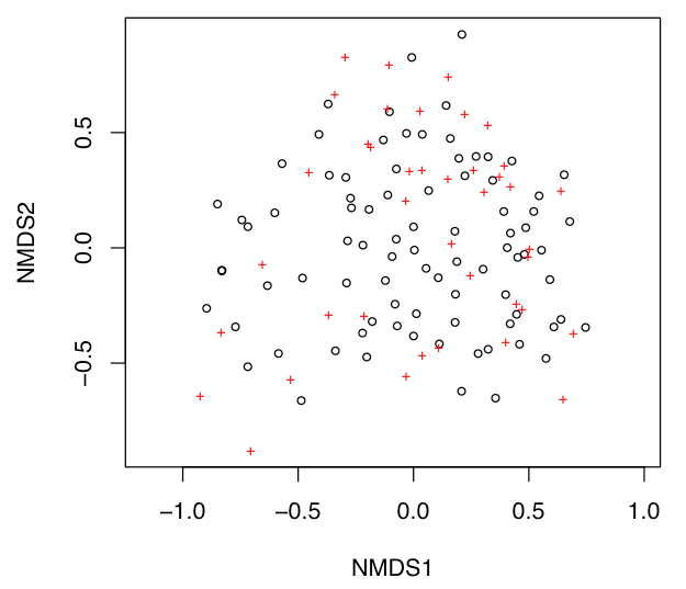
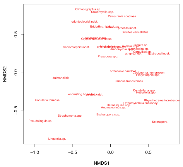
This default plot is uninformative because nothing is labeled, and you will usually want to customize an NMS plot. For example, it is often useful to display only the species or only the sites, which is done by setting display. It also helps to show the labels for the species or sites, which is done by specifying type="t", although crowding of labels is commonly a problem.
plot(nms, type="t", display=c("species"))
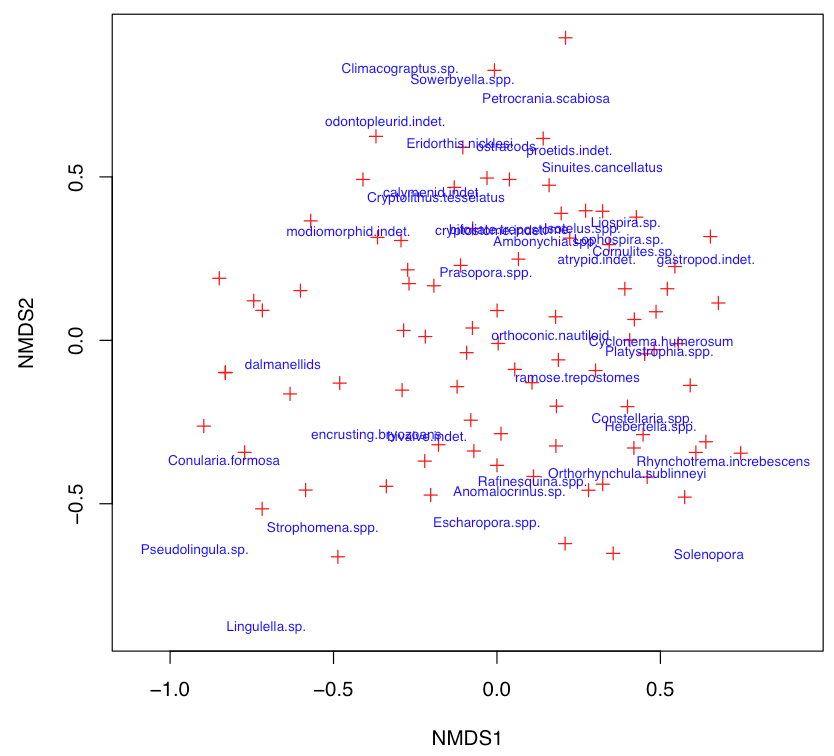
Customized NMS plots usually are better ways to plot the NMS results than the default plot. These are often customized like other bivariate plots by setting type="n" and plotting points and labels separately. If the labels are too crowded, setting cex to a value less than 1 will reduce the size of symbols and text. The choices parameter specifies which NMS axes to plot.
plot(nms, type="n")
points(nms, display=c("sites"), choices=c(1, 2), pch=3, col="red")
text(nms, display=c("species"), choices=c(1, 2), col="blue", cex=0.7)
For congested plots, the following code will display a plot with symbols for both samples and variables. Click on individual points that you would like identified. Press the escape key when you are done selecting your points to see their identities.
fig <- ordiplot(nms) identify(fig, "spec")
Example: Non-ecological data
NMS can also be performed on non-ecological data, but with several differences:
- First, the default distance metric (bray) is appropriate only for ecological data, in which species show a modal (not linear) response to environmental variables. In most cases with non-ecological data, the distance parameter should be set to euclidean.
- Second, the default data transformation that is appropriate for ecological data must be turned off by setting autotransform=FALSE and noshare=FALSE.
- All data values must be positive to calculate variable scores (called species scores). To do this, you will need to add a constant to each variable. The minShift() function shown below will do this by adding the absolute value of the minimum value for each variable. By doing this, the smallest value will be zero and all other values will be positive. Finally, to get variable scores, set wasscores=TRUE.
Prepare the data
Using the Nashville carbonates data set used in the principal components lecture (nashvilleCarbonates.csv), an NMS can be performed and plotted, resulting in a similar configuration of sample points. First, read the data, cull it, and apply data transformation, ending with one that ensures that all data values are positive. In this case, we remove column 1 because it is stratigraphic position (not a geochemical measurement) and we apply a log transformation to the elemental abundances.
nashville <- read.table("NashvilleCarbonates.csv", header=TRUE, row.names=1, sep=",") geochem <- nashville[ , -1] geochem[ ,3:8] <- log10(geochem[ , 3:8])
Because metaMDS wants all values to be positive (it is set up for ecological data, where a species abundance cannot be negative), we must shift all our values to positive ones. To do this, we create a function that adds the absolute value of the smallest value for each variable to all observations of that variable. Doing this causes the smallest value to be zero and all other values to be positive.
minShift <- function(x) {x + abs(min(x))} geochem <- apply(geochem, 2, minShift)
Run the NMS
Run the ordination and display the results.
chemNMS <- metaMDS(geochem, distance="euclidean", k=3, trymax=50, autotransform=FALSE, wasscores=TRUE, noshare=FALSE) chemNMS
Plot the scores
Plotting the data is easier if the sample and variable scores are extracted from the oridination.
variableScores <- chemNMS$species sampleScores <- chemNMS$points
To code the points by their formation, make logical vectors that describe the formation. This makes the subsequent code easier to read and less error-prone.
Carters <- nashville$StratPosition < 34.2 Hermitage <- nashville$StratPosition > 34.2
Make an empty plot, and add the points, color-coded by formation. Also, add color-code labels instead of a legend.
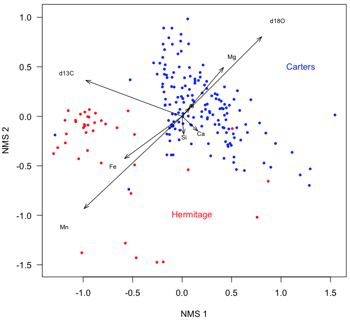
plot(sampleScores[, 1], sampleScores[, 2], xlab="NMS 1", ylab="NMS 2", type="n", asp=1, las=1) points(sampleScores[Carters, 1], sampleScores[Carters, 2], pch=16, cex=0.7, col="blue") points(sampleScores[Hermitage, 1], sampleScores[Hermitage, 2], pch=16, cex=0.7, col="red") text(1.2, 0.5, "Carters", col="blue") text(0.1, -1.0, "Hermitage", col="red")
Add vectors for the variables. The scaling factor textNudge ensures that the labels are plotted slightly before the tips of the arrows.
arrows(0, 0, variableScores[, 1], variableScores[, 2], length=0.1, angle=20) textNudge <- 1.2 text(variableScores[, 1]*textNudge, variableScores[, 2]*textNudge, rownames(variableScores), cex=0.7)
What to report
When reporting a non-metric multidimensional scaling, always include at least these items:
- A description of any data culling or transformations used before the ordination. State these in the order that they were performed.
- The distance metric, number of random restarts, and the specified number of axes.
- The value of stress.
- A table or plot of variable scores that shows how each variable contributes to each axis of the NMS.
- One or more plots of sample scores that emphasize the interpretation of the axes, such as color-coding samples by an external variable.
NMS results can be complex, and it is important to remember the GEE principle in your writing, which stands for Generalize, Examples, Exceptions. Begin each paragraph with a generalization about the main pattern shown by the data. Next, provide examples that illustrate that pattern. Cover exceptions to the pattern last. For example, you might do this with one paragraph on the variable scores for axis 1, then with one paragraph on the sample scores for axis 1, followed by two similar paragraphs on axis 2. If you do this in all your writing about data, not just NMS, it will be much easier for your readers to follow.
References
Holland, S.M., and M.E. Patzkowsky, 2004. Ecosystem structure and stability: middle Upper Ordovician of central Kentucky, USA. Palaios 19:316–331.
Legendre, P., and L. Legendre, 1998. Numerical Ecology. Elsevier: Amsterdam, 853 p.
McCune, B., and J.B. Grace, 2002. Analysis of Ecological Communities. MjM Software Design: Gleneden Beach, Oregon, 300 p.
