Nonlinear Regression
What makes an equation nonlinear?
A linear equation is any equation of the form y = ax + bz, that is, y equals the sum of a set of one or more coefficients, each multiplied by a variable. Such an equation is said to be linear in its parameters (the coefficients a and b in this example) and its variables (here, x and z). Any equation that cannot be put into this form is non-linear.
Some equations may not appear to be linear at first glance, but with a simple substitution, can be placed in linear form. For example, the equation y = ax + bx2 is linear because one could define a new variable z=x2, substitute it, and convert the equation to y = ax + bz. Likewise, y = ax2 + cex is also linear because, with two substitutions, w=x2 and z=ex, the equation becomes y = aw + cz and is now in linear form.
Some equations cannot be recast into linear form by substitutions. In situations like this, we must perform nonlinear least-squares regression, and this is easily done in R with the nls() function (for nls, think non-linear least squares).
Chapter 20 of The R Book by Michael J. Crawley is an excellent treatment of non-linear regression, and it includes a helpful table (20.1) of twelve common non-linear functions. If you need to fit a non-linear function, start with this chapter.
Explained variance
The nls() function does not produce coefficients of determination (R2), but the following r2nls()function will calculate a coefficient of determination for any model produced by nls(). This function uses the definition of the coefficient of determination, that is, one minus the sum of squares of the residuals divided by the total sum of squares.
r2nls <- function(model) { residuals <- residuals(model) y <- fitted(model) + residuals ssResiduals <- sum(residuals^2) ssTotal <- sum((y - mean(y))^2) rsq <- 1 - ssResiduals/ssTotal return(rsq) }
Fitting a nonlinear regression in R
Michaelis-Menten kinetics
One common non-linear equation is the Michaelis-Menten function, which is used in chemistry to describe reaction rate as a function of concentration. The Michaelis-Menten function is characterized by a steep rise that gradually flattens into a plateau. Initially, small increases in concentration cause a substantial increase in reaction rate, but additional increases in concentration cause progressively smaller increases in reaction rate. Eventually reaction rate plateaus and does not respond to increases in concentration. The Michaelis-Menten function has this form:
where r is the growth rate (the dependent variable), C is the concentration (the independent variable), Vm is the maximum rate in the system, and K is the concentration at which the reaction rate is half of the maximum (Vm/2). Thus, given a series of specified concentrations and the rates measured for each, the regression will find the best-fit coefficients Vm and K. We want to estimate these coefficients and the uncertainty in those estimates (i.e., confidence intervals).
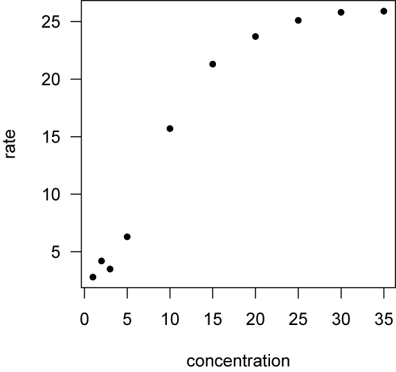
To fit this model, begin by entering the data (kinetics.txt) and plotting it. The data frame contains two variables, concentration and rate.
kinetics <- read.table("kinetics.txt", header=TRUE, sep=",") attach(kinetics) plot(concentration, rate, las=1, pch=16)
The shape of this relationship suggests that the Michaelis-Menten function might be a good model.
To fit the function, use nls(), which takes two arguments. The first argument is the model formula, specifying that the rate is a function of Vm multiplied by concentration, divided by the sum of K and concentration. Notice that unlike lm(), nls() does not need the I() function to specify that arithmetic operators ( *, /, +, etc.) should keep their algebraic interpretations. The second argument provides the fitting process with a starting estimate, the initial guesses for Vm and K; these are supplied as a list.
mmModel <- nls(rate ~ Vm * concentration / (K + concentration), start=list(Vm=30, K=25))
After fitting the model, its output is viewed with summary(). The fitted values of Vm and K can be extracted with the coef() function and their confidence intervals with the confint() function.
summary(mmModel) coef(mmModel) confint(mmModel)
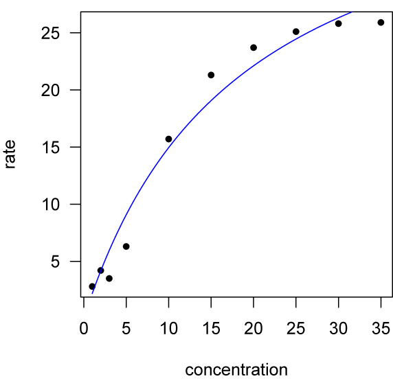
Adding the fitted function to our data plot takes a couple of steps. First, create a range of concentrations over which to evaluate the function, then evaluate the function over that range (that is, calculate the predicted rates at those concentrations), and finally add the points to the plot with the points() function. One might be tempted to evaluate the function by extracting the coefficients for the model and writing out the model, but it is simpler and less error-prone to use predict().
x <- seq(min(concentration), max(concentration), length=100) y <- predict(mmModel, list(concentration=x)) points(x, y, type="l", col="blue") detach()
Logistic growth
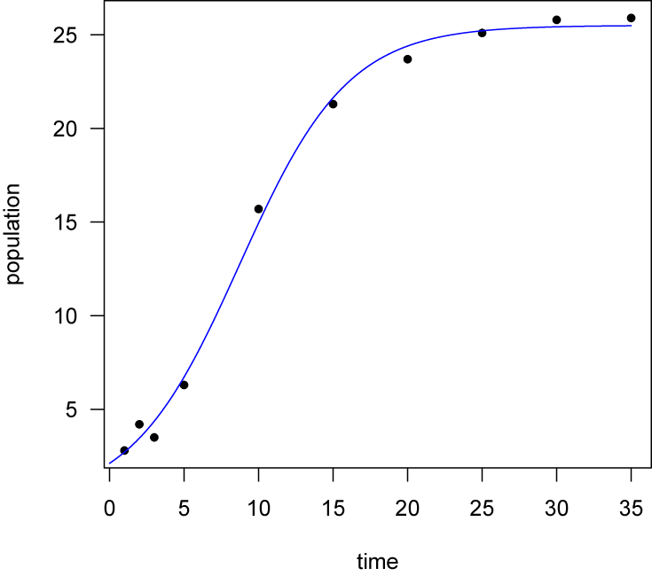
Another common model is used in biology to model the logistic growth of a population. Logistic growth is characterized by slow initial growth, followed by a period of rapid growth, and concluding by a period of slowing growth. This history produces the characteristic sigmoidal (s-shaped) relationship of logistic growth. The model can be written as

where P is population size (the dependent variable) and t is time (the independent variable). The three coefficients of the logistic model, Po (initial population size), r (growth rate), and K (carrying capacity, or final population size), are fitted by the regression.
Start as always by plotting the data (popGrowth.csv). The data frame contains two columns, population and time.
popGrowth <- read.table("popGrowth.csv", header=TRUE, sep=",") attach(popGrowth) plot(obsTime, population, las=1, pch=16, xlab="time")
Use the nls() function to fit the model, and supply initial guesses for the logistic parameters. These initial guesses might be made from another study that has fitted a logistic model to similar data.
logisticModel <- nls(population~K/(1+exp(Po-r*obsTime)), start=list(Po=5, r=0.211, K=5))
Non-linear fits can be sensitive to the initial guesses. If these initial guesses are poorly chosen, you may get a singular-gradient error
For this data, the initial population size seems close to zero, so zero is a reasonable initial guess for Po. The plot appears to plateau near 30, so that makes a good initial guess for K. To get an initial guess for r, select a point in the middle of the data set, substitute values of P and t into the equation, along with the initial guesses for Po and K, and solve for r. The model can then be specified with these appropriate guesses for the parameters, likely with better results.
logisticModel <-nls(population ~ K / (1 + exp(Po - r * obsTime)), start=list(Po=0, r=0.211, K=30))
As usual, view the results of the regression with summary(), the fitted parameters with coef(), and the confidence intervals with confint().
summary(logisticModel) coef(logisticModel) confint(logisticModel)
As in the Michaelis-Menton example, adding the fitted curve requires evaluating the function over the range of the data, and adding it with the points() function. The easiest way to evaluate the fitted function is with predict().
x <- seq(min(time), max(time), length=100) y <- predict(logisticModel, list(obsTime=x)) points(x, y, type="l", col="blue")
The added step of finding good starting parameters can be bypassed by using what is called a self-starting nls logistic model, using the SSlogis() function. This useful function creates an initial estimate of the parameters, which can then be fed to the nls() function to find the best-fit logistic equation. The SSlogis() function fits a slightly different parameterization of the logistic function:

where Asym is the carrying capacity, xmid is the x value at the inflection point of the logistic curve, and scal is a scaling parameter for the x-axis. These parameters are easily converted to the first form of the logistic model described above.

logisticModelSS <- nls(population~SSlogis(obsTime, Asym, xmid, scal)) summary(logisticModelSS) coef(logisticModelSS) detach()
Similar self-starting models are also available for the Michaelis-Menten model and several other functions, and they are all part of the built-in stats package.
References
Crawley, M.J., 2013. The R Book. Wiley: Chichester, 1051 p.
