Quantile–Quantile (Q-Q) Plots
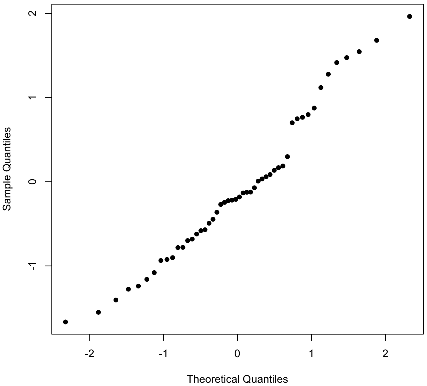
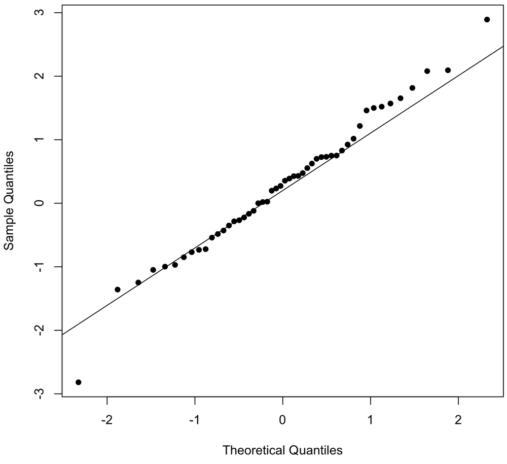
Quantile–quantile plots are a common way of comparing distributions, and they are especially common for assessing visually whether a distribution is normal. What they plot are the quantiles from the observed distribution against those from a theoretical distribution (often a normal distribution). If the observed distribution is of the same type as the theoretical distribution, the points will fall close to a line, as for these data, simulated from a normal distribution.
x <- rnorm(50) qqnorm(x, pch=16, main="") qqline(x)
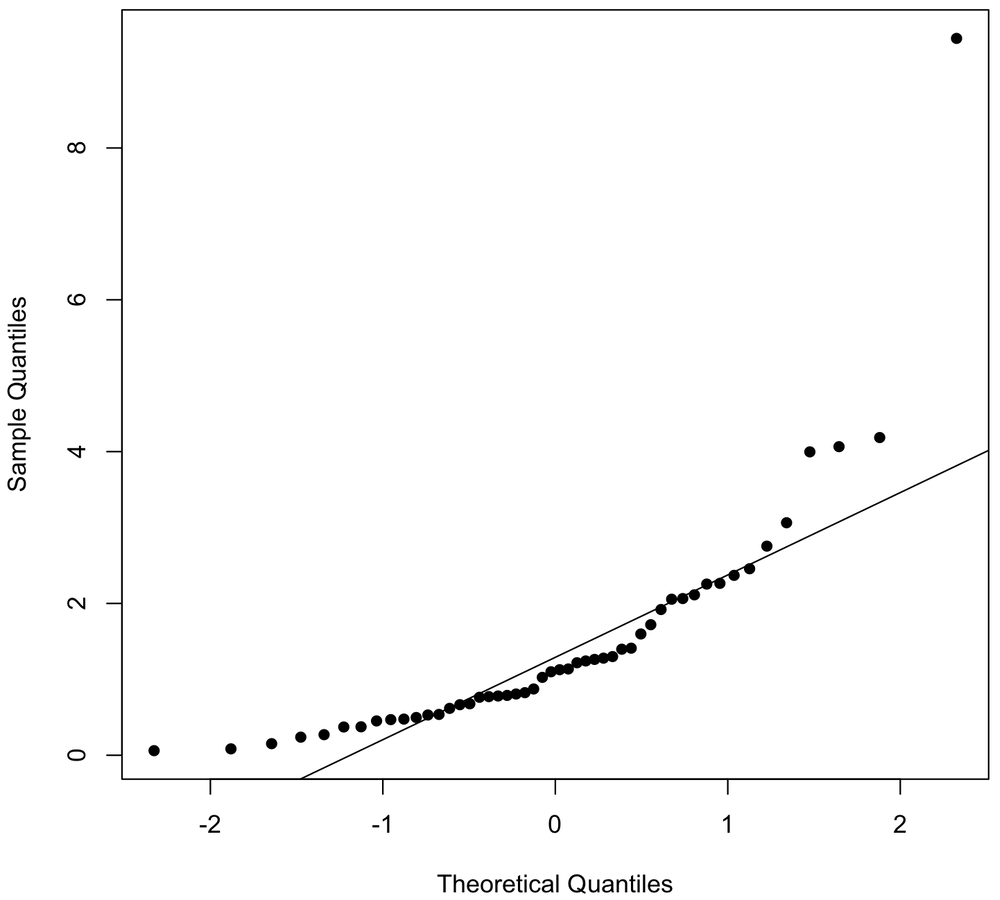
In this example, the data come from a log-normal distribution, so the points on the Q-Q plot strongly deviate from a line.
x <- rlnorm(50) qqnorm(x, pch=16, main="") qqline(x)
How a Q-Q plot is constructed
The key to understanding these plots is the idea of a quantile, which measure the proportion of the data that falls below a certain value. For our data, this is easily calculated by sorting the data in ascending order. For each data point, we then count the number of data points at or equal to that value, and divide that by the total number of data points. For example, if we have twenty data points, this would give a value for the smallest data point would of 1/20, or 0.05; for the second smallest data point, the proportion would be 2/20, or 0.10; and for the largest data point, it would be 20/20, or 1.0. The observed values are the sample quantiles corresponding to these proportions.
n <- 50 x <- sort(rnorm(n)) # Simulating some data proportions <- (1:n)/n
For the theoretical distribution, we can find the values of the theoretical distribution that correspond to these proportions by integrating from the left side of the distribution until we reach that proportion. For a normal distribution, the theoretical quantiles can be found for our 20 observations with R’s qnorm() function:
quantiles <- qnorm(proportions)
A Q-Q Plot plots the sample quantiles (x) versus the theoretical quantiles (quantiles):
plot(quantiles, x, pch=16, xlab="Theoretical Quantiles", ylab="Sample Quantiles")
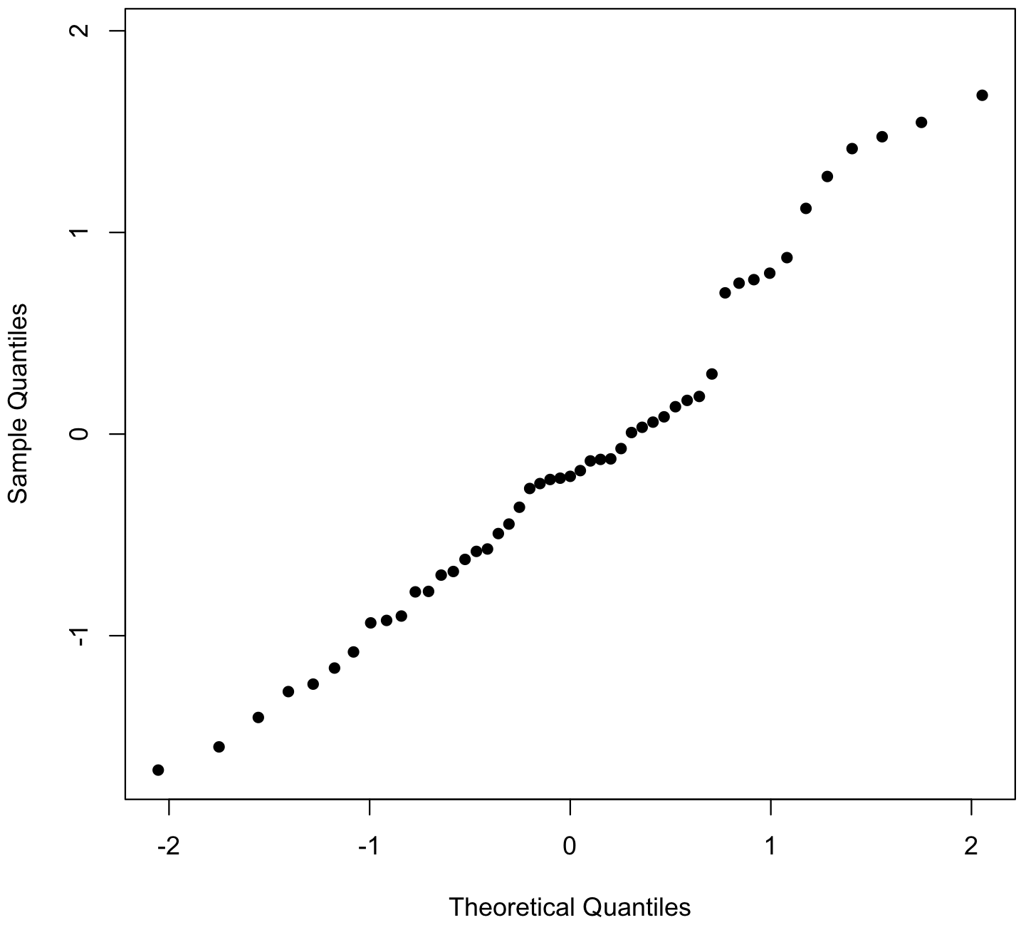
This is the same as if we simply called qqnorm() on our data:
qqnorm(x, main="", pch=16)