Resampling Methods
We can encounter several problems with traditional parametric and non-parametric statistical methods. For example, our sample size may be too small for the central limit theorem to ensure that sample means are normally distributed, so classically calculated confidence limits may not be accurate. We may not wish to resort to non-parametric tests that have low power. We may be interested in a statistic for which the underlying theoretical distribution is unknown. We cannot calculate confidence intervals, p-values, or critical values without a distribution.
Resampling methods are one solution to these problems and have several advantages. They are flexible and intuitive. They often have greater power than non-parametric methods and sometimes parametric methods. Two of them (bootstrap, jackknife) make no assumptions about the shape of the parent distribution other than that the sample is a good reflection of that distribution, which it will be if you have gathered a random sample through good sampling design and if your sample size is reasonably large enough. These same two can also be applied to any problem, even when there is no theoretical distribution of the statistic. They are less sensitive to outliers than parametric methods. Ties (observations having the same value) do not pose the problem they do in non-parametric methods.
Resampling methods have few drawbacks. The main difficulty is that they can be more difficult to perform than a traditional parametric or non-parametric test. They are less familiar to some scientists, which can cause problems in their acceptance, although this is becoming less of an issue. The methods are less standardized than parametric and non-parametric tests and are sometimes computationally expensive.
There are four main types of resampling methods: randomization, Monte Carlo, bootstrap, and jackknife. These methods can be used to build the distribution of a statistic based on our data, which can then be used to generate confidence intervals on a parameter estimate. They can alternatively be used to build the distribution of a statistic based on a null hypothesis, which can be used to generate p-values or critical values.
Monte Carlo
Monte Carlo methods are typically used in simulations where the parent distribution is either known or assumed. Without saying so, I have used Monte Carlo methods all semester to illustrate how statistical techniques work.
For example, suppose we wanted to simulate the distribution of an F-statistic for two samples drawn from a normal distribution. We would specify the mean and variance of the normal distribution, generate two samples of a given size, and calculate the ratio of their variances. We would repeat this process many times to produce a frequency distribution of the F-statistic, from which we could calculate p-values or critical values.
Here is an example of a Monte Carlo in R. The first block of code creates a function that calculates the F ratio of two samples, with sample sizes n1 and n2. The second block of code declares the sample sizes we want to simulate and calls our function many times to build a distribution of F values.
simulateOneF <- function(n1, n2) { data1 <- rnorm(n1) data2 <- rnorm(n2) F <- var(data1) / var(data2) return(F) } n1 <- 12 n2 <- 25 F <- replicate(n=10000, simulateOneF(n1, n2))
We can calculate a p-value by finding the percentage of our F values that equal or exceed an observed F-statistic (3.5 in this example):
Fobserved <- 3.5 pValue <- length(F[F >= Fobserved]) / length(F) pValue
This finds the proportion of F-values that exceed the observed of F of 3.5, so it is a one-tailed p-value. To obtain a two-tailed p-value, double this probability.
Because the p-value can be calculated like this for the expected distribution of any statistic, we can write a function that calculates the p-value for an statistic (observed) for any null distribution (nullDist) generated by a resampling method like the Monte Carlo:
pvalue <- function (observed, nullDist, tails=1) { nExtreme <- length(nullDist[nullDist>= observed]) nTotal <- length(nullDist) p <- nExtreme / nTotal * tails return(p) }
Calling this is simple: the first argument is the distribution provided by the Monte Carlo (or another resampling method), and the second argument is the observed statistic. By default, it will calculate a one-tailed (right-tailed) p-value; specify tails=2 for a two-tailed p-value. Calling a home-made function like this produces code that is simpler to read and more self-explanatory:
pvalue(Fobserved, F)
To summarize, there are three steps to a Monte Carlo:
- simulate observations based on a theoretical distribution
- repeatedly calculate the statistic of interest to build its distribution based on a null hypothesis
- use the distribution of the statistic to find p-values or critical values.
Randomization
Randomization is a simple resampling method, and a thought model illustrates the approach. Suppose we have two samples, A and B, on which we have measured a statistic (the mean, for example). One way to ask if the two samples have significantly different means is to ask how likely we would be to observe the difference in their means if the observations had been randomly assigned to the two groups. We could simulate that by randomly assigning each observation to groups A or B, calculating the difference of means, and repeating this process until we build up a distribution of the difference in means. By doing this, we are building the distribution of the difference in means under the null hypothesis that the two samples came from one population.
From this distribution, we could find critical values against which we could compare our observed difference in means. We could also use this distribution to calculate the p-value of the observed statistic.
The essential steps in randomization are:
- shuffle the observations among the groups
- repeatedly calculate the statistic of interest
- use that distribution of the statistic to find critical values or p-values
Here is an example of performing a randomization to evaluate the difference in means of two samples.
# The data x <- c(0.36, 1.07, 1.81, 1.67, 1.16, 0.18, 1.26, 0.61, 0.08, 1.29) y <- c(1.34, 0.32, 0.34, 0.29, 0.64, 0.20, 0.50, 0.85, 0.38, 0.31, 2.50, 0.69, 0.41, 1.73, 0.62) # Function for calculating one randomized difference in means randomizedDifferenceInMeans <- function(x, y) { nx <- length(x) ny <- length(y) # combine the data combined <- c(x, y) ncom <- length(combined) indices <- 1:ncom # initially assign all observations to y group group <- rep("y", ncom) # assign a subsample to to x group xsub <- sample(x=indices, size=nx) group[xsub] <- "x" # calculate the means meanX <- mean(combined[group=="x"]) meanY <- mean(combined[group=="y"]) differenceInMeans <- meanX - meanY return(differenceInMeans) } # Repeat that function many times to build the distribution diffMeans <- replicate(n=10000, randomizedDifferenceInMeans(x, y))
At this point, we could do several things. Because we have a distribution for the null hypothesis, we could compare the observed difference in means to the two-tailed critical values. From this, we could accept or reject the null hypothesis of no difference in means. The quantile() function makes finding the critical values easy.
alpha <- 0.05 observedDifference <- mean(x) - mean(y) quantile(diffMeans, alpha/2) quantile(diffMeans, 1-alpha/2)
It is often helpful to show the distribution with the critical and observed values. This allows readers to understand the distribution's shape and visualize where the observed value fell relative to the critical values.
hist(diffMeans, breaks=50, col="gray", xlab="Difference of Means", main="") observedDifference <- mean(x) - mean(y) abline(v=observedDifference, lwd=4, col="black") alpha <- 0.05 abline(v=quantile(diffMeans, alpha/2), col="red", lwd=2) abline(v=quantile(diffMeans, 1-alpha/2), col="red", lwd=2)
Instead of critical values, we could calculate the two-tailed p-value for our observed difference in means, using the p-value function we created above.
observedDifference <- mean(x) - mean(y) pvalue(diffMeans, observedDifference, tails=2)
Bootstrap
The bootstrap (Efron 1979) is a powerful, flexible, and intuitive technique for constructing confidence intervals. The name bootstrap comes from the idea of “lifting yourself up by your own bootstraps”: it builds the confidence limits from the distribution of the data. The main assumption is that the data are a good description of the frequency distribution of the population. It will be if you have collected a random sample through a good sampling design. Also, your sample size should not be so small that bad luck can create sample distributions unlike the population’s.
The principle behind a bootstrap is to draw a set of observations from the data to build a simulated sample of the same size as the original sample. This sampling is done with replacement, meaning that a particular observation might get randomly sampled more than once in a particular trial, while others might not get sampled at all. The statistic is calculated on this bootstrapped sample, which is repeated many times (thousands of times or more) to build a distribution for the statistic. The mean of these bootstrapped values is the estimate of the parameter.
The distribution of bootstrapped values is used to construct a confidence interval on the parameter estimate. There are several ways to do this, with the basic and percentile confidence intervals being the most common. Several more advanced approaches are not covered here, including expanded percentile, bootstrap t-table, bias corrected, and accelerated confidence intervals. Nathaniel Helwig provides a great comparative guide to all these approaches.
For the basic confidence interval, the mean and the standard deviation of the bootstrapped values are calculated, and these are used to calculate a standard t-score based confidence interval.

where θ̄ and sθ̄ are the mean and standard deviation of the bootstrapped statistic, and tα/2,ν is the two-tailed t-score for the significance level (α) and degrees of freedom (ν). The basic bootstrap confidence interval performs well when the distribution of the bootstrapped statistic is symmetric, which can be evaluated from a histogram of the bootstrapped statistic.
The second common approach is the percentile confidence interval. In this case, the confidence limits correspond to the points in the distribution of the bootstrapped statistic that correspond to α/2% and 1-α/2%. To do this, the bootstrapped values are sorted from lowest to highest. The 1-α/2% element (e.g. 0.025%) and the α/2% element (e.g., 0.975%) correspond to the lower and upper confidence limits. For example, if we calculated our statistic 10,000 times and wanted 95% confidence limits, we would find the elements at rows 250 and 9750 of our sorted vector of bootstrapped statistics. The quantile() function does all this automatically, saving us the trouble of sorting and finding the cutoffs. The percentile confidence interval performs well even when the bootstrapped statistic has an asymmetrical distribution.
The reliability of the bootstrap improves with the number of bootstrap replicates. Increasing the number of replicates increases the computation time, but this is seldom the problem that it was in the past.
Generalized bootstrap
A generalized bootstrap can be used in many situations, including where a statistic is based on one, two, or multiple variables. The function shown below can be easily adapted.
singleBootstrap <- function(x) { n <- length(x) # (1) obs <- 1:n # (2) sampledObs <- sample(x=obs, size=n, replace=TRUE) # (3) statistic <- sd(x[sampledObs]) # (4) return(statistic) } alpha <- 0.05 # (5) bootstrappedStat <- replicate(n=10000, singleBootstrap(x)) # (6) estimate <- mean(bootstrappedStat) # (7) lowerCL <- quantile(bootstrappedStat, alpha/2) # (8) upperCL <- quantile(bootstrappedStat, 1-alpha/2) # (9)
This example shows how to bootstrap a function (here, the standard deviation) that takes only one variable, x. In line 1, sample size (n) is calculated. In line 2, we create a vector of indices corresponding to each observation. In line 3, we sample those observations randomly to create as many observations as in our data set. Because we sample with replacement, any given bootstrap replicate may duplicate some observations and omit others, but these will change on every replicate. In line 4, we calculate the standard deviation of the bootstrapped sample with the sd() function. The last line of the function returns one bootstrapped statistic (here, a bootstrapped standard deviation).
Line 6 calls the bootstrap() function many times (10000 here) to produce a distribution of our bootstrapped statistic. The estimate of the population parameter (here, the population’s standard deviation) is calculated on line 7. The upper and lower percentile-based confidence limits are calculated on lines 8 and 9.
It is easy to modify this code to handle a different statistic that is based on one variable (median, mean, variance, etc.). Just replace the sd on line 4 with the name of the function you want to bootstrap.
For convenience, all these steps can be combined into a single function. The only arguments are the vector of data ( x ), the function to be bootstrapped ( FUN ), and optionally, the number of bootstrap iterations ( trials ) and the significance level ( alpha ). The function returns the bootstrapped estimate and the confidence limits.
oneVarBootstrap <- function(x, FUN, trials=1000, alpha=0.05) { singleBootstrap <- function(x, FUN) { n <- length(x) obs <- 1:n sampledObs <- sample(x=obs, size=n, replace=TRUE) statistic <- FUN(x[sampledObs]) return(statistic) } bootstrappedStat <- replicate(n=trials, singleBootstrap(x, FUN)) estimate <- mean(bootstrappedStat) lowerCL <- quantile(bootstrappedStat, alpha/2) upperCL <- quantile(bootstrappedStat, 1-alpha/2) results <- c(estimate, lowerCL, upperCL) names(results) <- c("estimate", "lower", "upper") return(results) }
To perform a 10,000-replicate bootstrap of the median value of iron at 99% confidence, the function would be called like this:
oneVarBootstrap(iron, FUN=median, trials=10000, alpha=0.01)
Two-variable bootstrap
Moreover, this procedure is easily adapted to bootstrap a function that takes two variables, such as a correlation coefficient. We’ll demonstrate this with a Spearman correlation coefficient because R’s cor.test() function does not provide a confidence interval on a Spearman correlation coefficient.
bootstrap <- function(x, y) { n <- length(x) # (1) obs <- 1:n # (2) sampledObs <- sample(x=obs, size=n, replace=TRUE) # (3) statistic <- cor(x[sampledObs], y[sampledObs], method="spearman") # (4) return(statistic) } bootstrappedStat <- replicate(n=10000, bootstrap(x, y)) # (5) estimate <- mean(bootstrappedStat) # (6) alpha <- 0.05 # (7) lowerCL <- quantile(bootstrappedStat, alpha/2) # (8) upperCL <- quantile(bootstrappedStat, 1-alpha/2) # (9)
The code from the one-variable bootstrap needs to be changed in only three places. The first is where we declare the bootstrap() function: we provide both variables needed to calculate the correlation coefficient. Second, we change in line 4 the name of the function (to cor), provide the function with the x and y values of our sampled observations, and specify that cor should calculate the Spearman coefficient. Last, we call the bootstrap() function with both of the variables it needs (line 5). So simple! This example also uses the percentile-based confidence limits.
Multi-variable bootstrap
The bootstrap for a function that takes on three or more variables can be done similarly. Modify the bootstrap() function to have arguments for each variable your function needs. If necessary, change line 1 to calculate the sample size from one of your variables if none are named x. Change line 4 so that your function is called with its necessary arguments. Change line 5 to call the bootstrap() function with the necessary data. This ease with which the bootstrap can be modified is one of the reasons it is such a widely used technique.
For some multivariate problems, the function to be bootstrapped may take a data frame as an argument, not individual variables (e.g., PCA and other ordinations, cluster analysis, etc.). In this case, the bootstrap() function will need more modification, but the principle is the same. To calculate confidence intervals, randomly sample rows from the data frame and use all the variables for those rows. If you want p-values or critical values, you will randomly select data for each variable, such that the data are now shuffled. In other words, you will build new observations that produce new random combinations of the variables drawn from the data.
Some methods (such as non-metric multidimensional scaling) do not allow identical cases (rows of data), which will cause a problem for a multivariate bootstrap. A common solution is to add a very small random number to each value as that case is selected, preventing the problem of identical cases. For example, if data values range from 1–10, the added random number could be on the scale of 0.001. This would be enough to prevent values from being identical but not enough to substantially alter the data or the results.
The boot package
The boot package can also be used to create bootstrapped estimates and confidence intervals. The advantage of the boot package is that it can compute five types of confidence intervals: first-order normal approximation (normal), basic bootstrap interval (basic), studentized bootstrap interval, bootstrap percentile interval (percentile), and adjusted bootstrap (BCa) interval (boosted). The studentized bootstrap interval is the method described above that uses t scores. The bootstrap percentile interval is described and demonstrated in code above, and the boot package replicates these results.
Performing the bootstrap with the boot package is straightforward; the details of performing the bootstrap and the confidence interval are hidden, however.
library(boot) # 1 mysd <- function(values, i) sd(values[i]) # 2 myboot <- boot(treeHeight, mysd, R=10000) # 3 myci <- boot.ci(myboot) # 4
Step #1 is to load the boot library. In step #2, you declare the function that will be bootstrapped. This function must be set up in this specific way; refer to the help page for the boot() function for more details. The first argument for the function will be the values (the data) to be bootstrapped, and the second argument will correspond to an observation number. Line #3 performs the bootstrap, 10000 times in this example. Step #4 calculates all the confidence intervals from the bootstrap. These confidence intervals can differ substantially.
For convenience, these steps can be combined into a single function. The only arguments are the vector of data ( x ), the function to be jackknifed ( FUN ), and optionally, the significance level ( alpha ). The theta notation inside the function is a common way of denoting the estimates. The function returns the jackknifed estimates (biased and unbiased), standard error, bias, and confidence limits.
Summary
To summarize, a bootstrap has three steps:
- simulate observations based on sampling with replacement from the data
- repeatedly calculate the statistic of interest
- use that distribution to estimate the parameter and a confidence interval
The bootstrap should be used with caution when the sample size is small because the data may not adequately represent the population’s distribution, violating the only assumption of the bootstrap.
The bootstrap is an incredibly versatile technique. All scientists should know how to implement one.
Jackknife
The jackknife is another technique for estimating and placing confidence limits on a parameter. The name refers to cutting the data because it removes a single observation, calculates the statistic without that one value, and then repeats that process for each observation (remove just one value, calculate the statistic). This produces a distribution of jackknifed values of our statistic, from which a parameter estimate and confidence interval are calculated.
Specifically, suppose we are interested in parameter K, but we have only an estimate of it (the statistic k) that is based on our sample of n observations.
Remove the first observation in the data to form the first jackknifed sample consisting of n-1 observations. Calculate the statistic (called k-i) on that sample, where the -i subscript means all the observations except the ith. From this statistic, calculate a quantity called the pseudovalue κi :

Repeat this process by replacing the first observation and removing the second observation to make a new sample of size n-1. Calculate the statistic and pseudovalue as before. Repeat this for every possible observation until there are n pseudovalues, each with sample size n-1. From these n pseudovalues, we can estimate the parameter, its standard error, and the confidence interval.
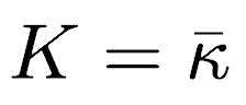
The jackknifed estimate of the parameter K is equal to the mean of the pseudovalues:
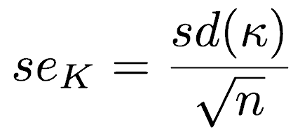
The standard error of K equals the standard deviation of the pseudovalues divided by the square root of sample size (n):
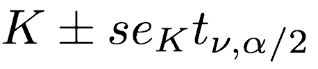
The jackknifed confidence limits are based on the estimate of K, the standard error, and the two-tailed critical t-score with n-1 degrees of freedom:
There are two caveats for the jackknife. First, the confidence intervals assume that the jackknifed statistic is normally distributed, which is justified by the central limit theorem for large samples. The central limit theorem may not assure normality if our sample size is small. Moreover, resampling methods assume that the data are a good reflection of the populations, and this is commonly not true when the sample size is small. Second, the pseudovalues are not independent, they are necessarily correlated.
Here is an example of how to jackknife a statistic; here, we will create a jackknifed estimated of standard deviation and the confidence limits on that estimate. This will be done on a vector of data ( x ).
Next, calculate the pseudovalues. First, we will get the sample size, calculate the statistic (stat) on the data, and make a vector to hold the pseudovalues. We loop through the data, removing each observation individually, calculate the statistic, then calculate the pseudovalue and store it. The for loop is one way to do this; the way it works is that it starts with i=1 (the first observation), incrementing i at each step, and ending when i=n. The same approach can be done with sapply(), but I think the loop is simpler to read and is not perceptibly slower.
n <- length(x) stat <- sd(x) # sd() will be jackknifed pseudovalues <- rep(0, n) for (i in 1:n { jackStat <- sd(x[-i]) # jackknife of sd() pseudovalues[i] <- stat - (n-1)*(jackStat-stat) }
From the statistic and the pseudovalues, we calculate the jackknifed estimate, standard error, and confidence limits.
estimate <- mean(pseudovalues) SE <- sd(pseudovalues) / sqrt(n) alpha <- 0.05 lowerCL <- estimate + qt(p=alpha/2, df=n-1) * SE upperCL <- estimate - qt(p=alpha/2, df=n-1) * SE
For convenience, these steps can be combined into a single function. The only arguments are the vector of data ( x ), the function to be jackknifed ( FUN ), and optionally, the significance level ( alpha ). The theta notation inside the function is a common way of denoting the estimates. The function returns the jackknifed estimates (biased and unbiased), standard error, bias, and confidence limits.
jackknife <- function(x, FUN, alpha=0.05) { n <- length(x) thetaHat <- FUN(x) thetaHatI <- rep(0, n) for (i in 1:n) { thetaHatI[i] <- FUN(x[-i]) } thetaHatDot <- mean(thetaHatI) bias <- (n-1) * (thetaHatDot - thetaHat) pseudovalues <- n*thetaHat - (n-1)*thetaHatI jackEstimate <- thetaHat jackEstimateBiasCorrected <- mean(pseudovalues) jackSE <- sqrt((n-1)^2/n * var(thetaHatI)) tCrit <- qt(p=alpha/2, df=n-1) lowerCL <- jackEstimateBiasCorrected + tCrit * jackSE upperCL <- jackEstimateBiasCorrected - tCrit * jackSE results <- c(jackEstimate, jackEstimateBiasCorrected, jackSE, bias, lowerCL, upperCL) names(results) <- c("estimate", "estimateBiasCorrected", "SE", "bias", "lowerCL", "upperCL") return(results) }
This function could be used to jackknife the standard deviation for a vector of iron values like this:
jackknife(iron, sd)
To summarize, the jackknife has three main steps:
- remove one data point, calculate the statistic and the pseudovalue
- repeat this process, leaving out one data point at a time to build a set of n pseudovalues
- use the pseudovalues to estimate the parameter and the uncertainty
Like the bootstrap, this approach could be modified to jackknife bivariate or multivariate data. The procedure is the same: remove one sample (a row in a data frame) at a time and calculate pseudovalues, from which jackknifed estimates, standard error, bias, and confidence limits are calculated.
References
Crowley, P. H. 1992. Resampling methods for computation-intensive data analysis in ecology and evolution. Annual Review of Ecology and Systematics 23:405–447.
Davison, A. C., D. V. Hinkley, and G. A. Young. 2003. Recent developments in bootstrap methodology. Statistical Science 18:141–157. This entire issue of Statistical Science is devoted to the bootstrap.
Efron, B. 1979. Bootstrap methods: another look at the jackknife. The Annals of Statistics 7:1–26.
