Variance
Understanding and characterizing variation in samples is an important part of statistics. Variation can be measured with several different statistics. Range, standard deviation, and variation are three of the most common.
Range is the difference between the largest and smallest values in a distribution and is calculated in R with range(). Because range tends to increase with sample size and because it is highly sensitive to outliers, it is often not a useful measure of variation. Range is also a biased estimator in that the sample range is nearly always smaller than the population range.
Variance is a much more useful measure of variation. The variance of a population is equal to the average squared deviation (difference) of every observation from the population mean. It is symbolized by a Greek lowercase sigma-squared (σ2).

Because the population mean is usually unknown, the sample variance is calculated as the sum of squared deviations of every observation from the sample mean, divided by the degrees of freedom. Doing this applies a penalty for using the sample mean to estimate the population mean. Sample variance is symbolized by a Roman lowercase s-squared (s2) for samples.

In R, sample variance is calculated with the var() function. In those rare cases where you need a population variance, multiply the sample variance by (n-1)/n. As the sample size gets very large, (n-1)/n converges on 1, so the sample variance converges on the population variance.
Because variance is the average squared deviation from the mean, the units of variance are the square of the original measurements. For example, if the length of cars is measured in meters, variance has units of m2. As a result, the units of variance are often not intuitive. This is solved by taking the square root of the variance, such that the quantity has the same units of variance. That’s standard deviation, the square root of variance. The sample standard deviation is calculated with the sd() function.
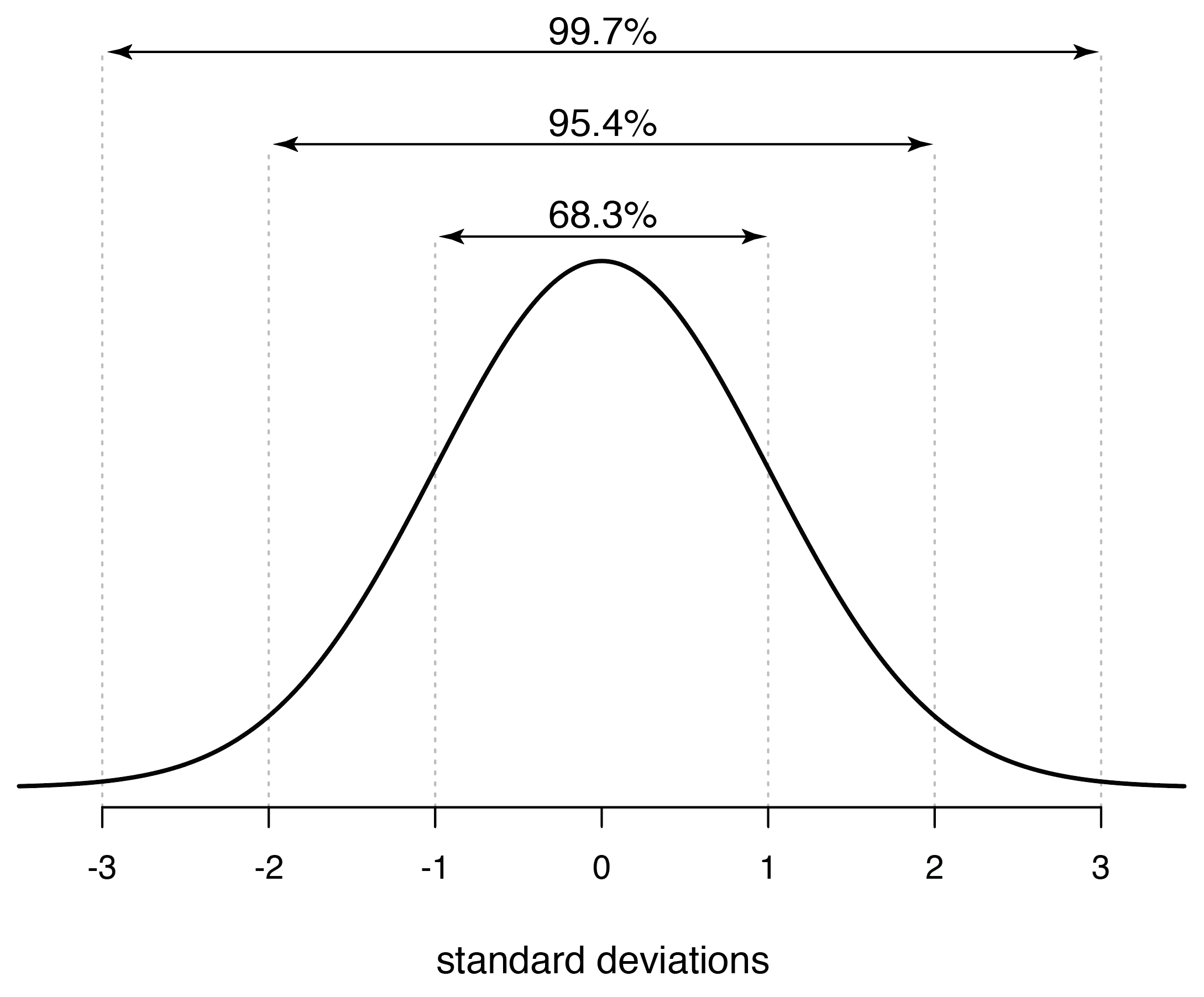
A normal distribution is scaled by the standard deviation, with 68.3% of the distribution within one standard deviation of the mean, 95.4% within two standard deviations of the mean, and 99.7% within three standard deviations (you can calculate these easily with the qnorm() function). These are good rules of thumb to remember, particularly that plus or minus two standard deviations encompasses roughly 95% of a normal distribution. This can give you an idea of how unusual and observation is, such as in a t-distribution, which is increasingly similar to a normal distribution at larger sample sizes.
The coefficient of variation is the standard deviation divided by the mean. As these have the same units, the coefficient of variation is a dimensionless number, which makes it a valuable way to describe variation. It is often used because the amount of variation is related to the average value of what is being measured, and this rescaling corrects for that.
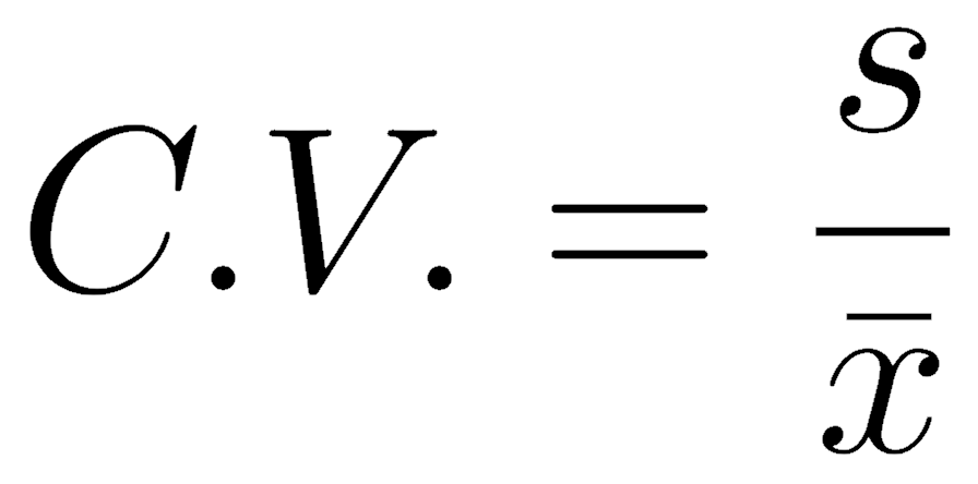
There is no built-in function for the coefficient of variation in R, but writing such a function is straightforward:
CV <- function(x) { sd(x) / mean(x) }
Comparing variances in two samples
To compare variances, we express them as a ratio, known as an F statistic. The F statistic is named for its discoverer, the biostatistician R.A. Fisher (of p-value and Modern Synthesis fame). It is therefore also called Fisher’s F.
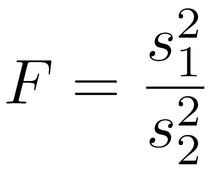
As with any statistic, we need to understand how it is distributed, and a thought experiment helps. Imagine two samples drawn from the same population; they ought to have similar variances, so the F statistic should generally be close to one, although it will differ for any pair of samples. For the simulation, we will assume that both samples are drawn from the same normally distributed population. We state the two sample sizes (n1 and n2), generate normally distributed values for each (using rnorm()), calculate their variances (with var()), and then measure the ratio of their variances. This is repeated many times (numTrials=10000) using the replicate() function, which saves those simulated F ratios to an object named F.
n1 <- 12 n2 <- 25 numTrials <- 10000 F <- replicate(numTrials, var(rnorm(n1))/var(rnorm(n2))) hist(F, breaks=50, col="salmon", main=paste("n1=",n1,", n2=",n2, sep=""))
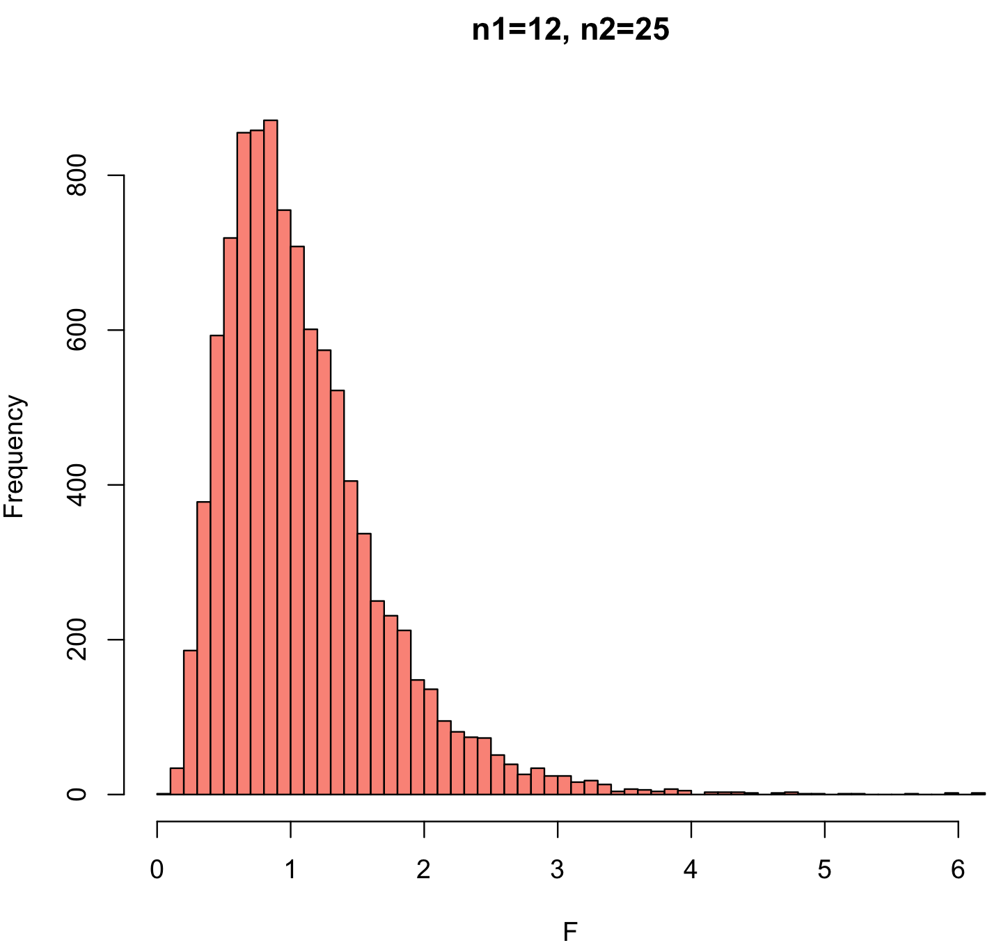
This distribution matches what we would expect. Two samples from the same population should typically have similar values, so the mode of the F-ratio is near 1. In some cases, the variance of one sample may be much longer than the other, and this creates the two tails of the distribution. Because variance is always positive, the smallest possible value of the F-ratio is 0 (when the numerator is zero, meaning that all the values are identical). The largest possible value would be positive infinity (when the denominator is zero). As a result, the left tail is short, and the right tail is long. The probability of generating such extreme F-ratios depends on the sample size of the two samples, so the shape of the F-distribution reflects the degrees of freedom for the numerator and for the denominator.
In practice, F distributions come from analytic solutions, not from simulations like this. Analytic solutions similarly assume that both samples come from normal distributions, which is an important consideration in applying the F distribution.
As with all distributions, R has four functions to explore the F distribution. These include df() to find the height of the distribution from F and the two degrees of freedom; pf() to obtain a p-value from an observed F and the two degrees of freedom; qf() to obtain a critical value from alpha and the two degrees of freedom; and rf() to obtain random variates from an F distribution from the two degrees of freedom. Here is the distribution we simulated above, but calculated analytically with df(). Our numerical simulation approximates the exact analytical solution well.
F <- seq(from=0, to=5, by=0.01) density <- df(F, df1=n1-1, df2=n2-1) plot(F, density, type="l", lwd=2, las=1)
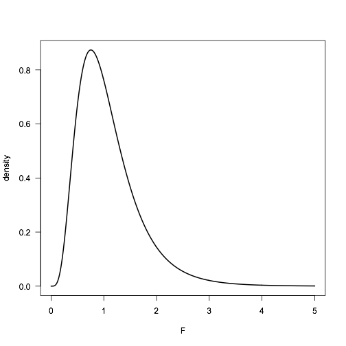
Once we have a statistic and the distribution of the expected values, we can place confidence limits on an F-ratio. We can also perform statistical tests on a null hypothesis of the F-ratio, and the null hypothesis is usually that the two samples were drawn from the same population or from populations with the same variance.
The F-test is based on two assumptions. The first is random sampling, an assumption common to all tests. The second is that both samples come from populations that are normally distributed. If your data are not normally distributed, a data transformation may help; if it doesn’t help, you will need to use a nonparametric test to compare the variances.
An F test is performed in R with the var.test() function. Here is a demonstration using two simulated data sets:
data1 <- rnorm(50, mean=3, sd=2) data2 <- rnorm(44, mean=2, sd=1.4) var.test(data1, data2)
This is by default a two-tailed test, and it does not matter which variance you put in the numerator and denominator. You can specify one-tailed tests with the alternative argument. You can also change the confidence level with the conf.level argument. The var.test() function produces the following:
F test to compare two variances data: data1 and data2 F = 1.8911, num df = 49, denom df = 43, p-value = 0.03519 alternative hypothesis: true ratio of variances is not equal to 1 95 percent confidence interval: 1.046032 3.380349 sample estimates: ratio of variances 1.891094
Because this example uses simulated data, you will likely get a slightly different answer every time you run this code. The ratio of variances (F ratio) is listed at the end of the output. The confidence interval on the ratio of variances is given on the seventh line. If you are performing a hypothesis test, report the values shown in the line beginning “F=”; be sure to include the F-ratio, both degrees of freedom, and the p-value. The results of this test could be stated succinctly as “The ratio of variances is 1.89 (95% C.I.: 1.05–3.38).”
Testing multiple variances: Bartlett test
Sometimes, you may need to compare the variances of multiple groups, and to do that, use Bartlett’s test for the homogeneity of variances. Like the F-test, Bartlett’s test is a parametric test: it assumes that the data are normally distributed. In R, a Bartlett’s test is run with bartlett.test(). Your data should be set up with the measurement variable in one vector and a grouping variable in a second vector. The test is run like this:
bartlett.test(measurementVariable, groupingVariable)
For example, suppose you are calculating alkalinity measurements in several streams and have multiple replicates in each stream. If you wanted to test that the variance in alkalinity is the same in all streams, your test would be called like this:
bartlett.test(alkalinity, stream)
The non-parametric Ansari-Bradley test
If your data are not normally distributed, first try a data transformation (such as the log transformation) to see if the distributions can be made normal. If a data transformation does not produce normality, you must use a non-parametric test, such as the Ansari-Bradley test.
The Ansari-Bradley test makes only one assumption: random sampling. It is called in R like this:
ansari.test(data1, data2)
The output consists of the AB statistic and a p-value. Like all non-parametric tests, confidence limits on a population parameter cannot be made.
Background reading
Read chapter 4 of Crawley, entering the code in R as always. Skim (or read, but do not get bogged down) the part on the bootstrap, a technique we will cover later.
