Problem Set 6: ANOVA
Conrad Labandeira and Nigel Hughes independently studied the Late Cambrian trilobite Dikelocephalus for their master’s theses. Each came to the same conclusion, that Ulrich and Resser, who described many species of that genus in the early 1900’s, had vastly oversplit the genus and that many of the species could not be distinguished. For this week’s problem set, you will examine a small portion of the data they analyzed (Journal of Paleontology 68:492–517).
In the trilobites4 data set are two measurements of the free cheek (the side of the head) for four species of Dikelocephalus. Labandeira and Hughes called these measurements omega and sigma; both are measured in centimeters (cm). They measured many other aspects of these trilobites and for many other species, but to keep this problem tractable, you will examine only omega and only on four of the species (D. edwardsi, D. gracilis, D. raaschi, and D. subplanus).
In this problem set, you want to evaluate whether these four species can be distinguished on the basis of this one measure. This is a problem of central tendency: how different are these species? If the central tendencies of these measures are similar, it will be hard to distinguish the species, but if the central tendencies are substantially different, it should be possible to tell them apart. Some species may be distinguishable, and others may not.
In your work, remember three things:
- Plots should follow the instructions of problem sets 4 and 5.
- Answers to questions should follow the instructions given in problem sets 4 and 5.
- When asked to state the results of a statistical test, follow standard practice, in which you provide parenthetical numerical support for your statements in the correct format.
Part 1
Import the trilobites4 data and save it to an object named trilobites. One of the columns in this data is a categorical (nominal) variable of species names. Nominal variables should be set up as factors rather than strings; do this by setting stringsAsFactors=TRUE as you import the data.
Use the appropriate command to view the structure of this data frame.
Use the appropriate command that allows you to call variables by name without using dollar-sign notation. Remember to undo this command as the last command of this problem set.
Last, you want to see the names of every species; use levels() to see all possible values of the species factor.
Part 2
Visualize how omega is distributed for each species, using one plot constructed in one line of code; this is plot 1. Use stripchart() with the data (omega) grouped by species. Hint: stripchart(y~x) will plot the variable y grouped by the variable x (often a factor). Use solid black circles for the plotting symbol. Give an appropriate x-axis label following the convention for indicating the units. Rotate the y-axis labels. As there is a too much white space on the default plot size, make the plot 7" wide and 4" tall. Turn off drawing the frame around the plot, which will make the plot less crowded.
The first time you make this plot, you should notice that the species names are truncated. To avoid this, you need to call par() before you create the plot and set the mar() argument to create more space on the left side of the plot. The easiest way is to use the default values from the help page and modify only the one value just enough so that the species names are not truncated. This call to par() and mar() should be invoked after you create the pdf file but before you create the strip chart.
Question 1: Consider what the plot shows before doing the statistical analyses. Does the mean value for all four species appear to be about the same, or do any of the species look different? Eyeball any estimates of the means, but do not calculate them.
Part 3
A common way in which data like this is evaluated is to test in one step whether the means of all of the species are statistically indistinguishable, and this is usually done with an ANOVA. Before you can run an ANOVA (or any statistical test), you must verify its assumptions. Remember, assumptions are requirements of the tests; they are things you must demonstrate, not things that you should assume.
Question 2: The first requirement of an ANOVA is that the data are normally distributed. Based on a visual examination of your stripchart, and considering the small sample size, is omega roughly symmetrically distributed for each species or is it clearly asymmetrical for some species (if so, which ones)? Because the data set is small, you should be concerned only about strong departures from symmetry. Although omega for one of the species has a strongly bimodal distribution, you should not be concerned with that for this problem set.
The second requirement of an ANOVA is that the variance for each species is the same, or more accurately, that they are indistinguishable. Use the appropriate test that lets you compare the variances of omega on all four groups in one simple line of code.
Question 3:Based on the test results, should you accept or reject the null hypothesis that the variances of the species are indistinguishable?
Question 4: State whether the assumptions of normality and homoscedasticity (equal variances) been met for an ANOVA on omega.
Part 4
Normally, you would proceed to the ANOVA only if the assumptions of the test were met. In this case, I want you to perform the ANOVA regardless of whether you think the assumptions were met.
Run an ANOVA using aov() on omega as a function of species. So that you can see the full ANOVA table, save the results to an object called omegaANOVA, then display this table with the appropriate command.
Question 5: Do the results indicate that the mean value of omega is indistinguishable among all four species; in other words, do you accept or reject the null hypothesis? Remember to provide parenthetical support, a summary of your statistical test. If you concluded in question #4 that the assumptions of the ANOVA were not valid, explain in an additional sentence how this affects the interpretation of the test results.
Part 5
Regardless of the results of the test, you need to evaluate effect size. One important measure of this is η2, the proportion of the variance explained by differences among species. Several lines of code are given in the lecture notes for calculating this. Convert that code into a function called etaSquared. The only argument it should take is an ANOVA model, and it should return the proportion of variance labeled by the source. Be sure that the function relies only on what is passed to it in the arguments; the argument should be generic in that it should not be specific to the ANOVA you just ran. I will test your function on a data set that you cannot see, so you should test it to make sure it works. Do not include your tests of the function in the code you turn in.
Run your function on the ANOVA model you created in Part 4.
Question 6: What proportion of the variance in omega is explainable by species, and what proportion is unexplained?
Part 6
Given the result in Part 4, you should evaluate which species can be distinguished from the others. Run TukeyHSD() on the ANOVA model from Part 4.
Question 7: Based on the Tukey’s Honestly Significant Difference test, which species can be distinguished using omega, and which cannot? Do not report this one species pair at a time; instead, study the results and summarize the complete pattern in one sentence. You do not need to provide parenthetical numerical support for this question. If you were reporting these results in a manuscript, you would convert the output of your test to a table or figure and cite that parenthetically as support, but you will not do that here.
Part 7
The problem with the Tukey HSD approach is that it still does not tell us what we are most interested in, the mean omega for each species and our uncertainty in those means. To generate these confidence intervals, you will use the t.test() function. Call this function on omega for each species individually (that is, in four lines of code), assigning the result for each to an object named for the species. You will need to specify the values of omega to use with a logical test for each species.
Next, skip a line, then display the estimate and the confidence interval for one of the species, using two successive lines of code. Round both sets of values to a consistent and reasonable number of significant figures based on the data. Refer to the help page for t.test() to see how to extract (using $ notation) the estimate and the confidence interval from the result (called the value on the help page). Experiment with displaying the confidence limits so that only the confidence limits are shown, not the confidence level. There is a very simple way to do that that involves adding only a few characters after the closing parenthesis for round().
Skip a line, then do the same two lines of code for the next species; repeat this so that the mean omega and its confidence limits are displayed for all four species.
Question 8: Compare the four sets of confidence intervals on mean omega you just calculated. Based on whether these confidence intervals overlap, which species can be distinguished based on omega? I recommending sketching these to visualize how they compare. State your answer succinctly, similar to how you answered Question 7.
Question 9: Do these two approaches (Tukey HSD vs. confidence intervals) lead you to the same conclusion about which species can be distinguished?
Bonus (up to +5 points)
While talking about confidence limits with a friend (as you do), they sketch on a napkin an effective way to plot them. Here’s their sketch, coffee stain and all.
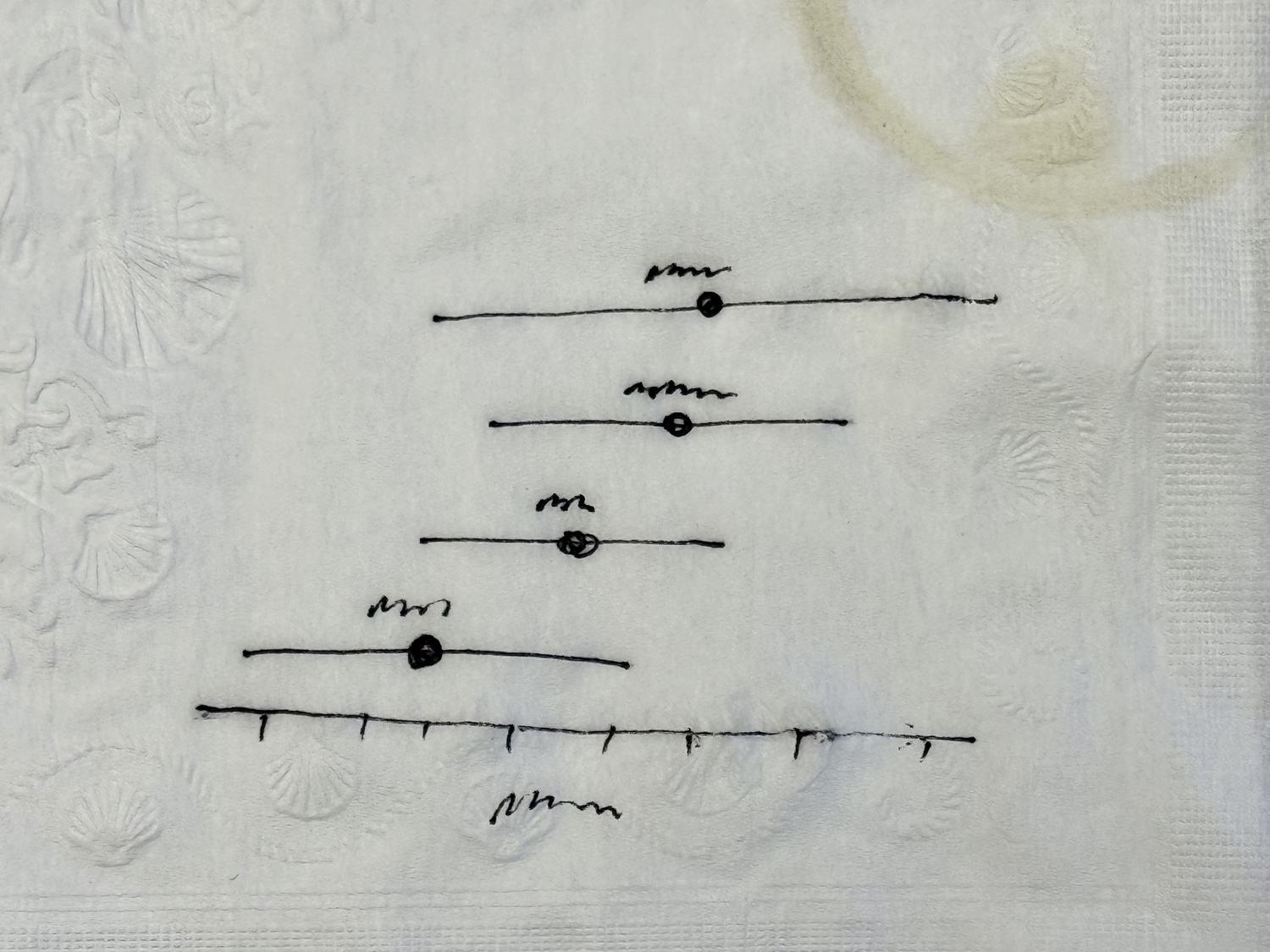
The squiggles are the x-axis label and the names of each species, placed just above the mean values.
Create this plot with your estimates and confidence intervals for the four species. This can be done with the plot(), points(), segments(), and text() commands. To help with grading, use your first name for the main argument to plot().
I will evaluate your figure based on its correctness, effectiveness in conveying the main point of the data, and our lecture about figure design. I’ll assess your code based on its understandability, simplicity, and conformance to the style guidelines used in this course. Your work should be your own.
If use a GPT to make this plot, you must acknowledge the assistance by submitting the complete transcript in a separate Word or PDF file (named hollandGPT.pdf or hollandGPT.doc, substituting your name). A GPT is not necessary — this is not a hard problem — and you will build your R skills faster if you do not use one here.
As usual, include this code in your main .R file. In addition, put the code for just this plot in a separate .R file with a name in the pattern of hollandPlot.R, where you substitute your name. This file should begin with a comment line with your name, followed a blank line, then just the commands for creating this bonus plot. I will not run this file; it is only to help me with grading.
Submitting your problem set
Format your commands file following the standard instructions. E-mail your commands file to stratum@uga.edu. The subject of your email should be 8370 problem set 6. If you complete the bonus, include the additional file(s) I request. This problem set is due Monday, 13 October.
