Covariance and Correlation
We frequently work with two variables simultaneously and want to understand their relationship. For this, there are two related yet distinct goals. The first is to understand the strength of the relationship between them, called correlation. The second is to know the mathematical function that describes the relationship, and can be used to make predictions; finding this relationship is called regression. We will cover these two topics separately in the next two lectures.
There are two common types of correlation, one describing the linear relationship and one describing the monotonic relationship. As you might guess, a linear relationship is one described by a line. A monotonic relationship is where one variable consistently increases or decreases as the other increases, although the relationship might not be linear (e.g., exponential). To measure the linear correlation, we start with the concept of covariance.
Covariance
Covariance is based on the sum of products, which is analogous to the sum of squares used to calculate variance:
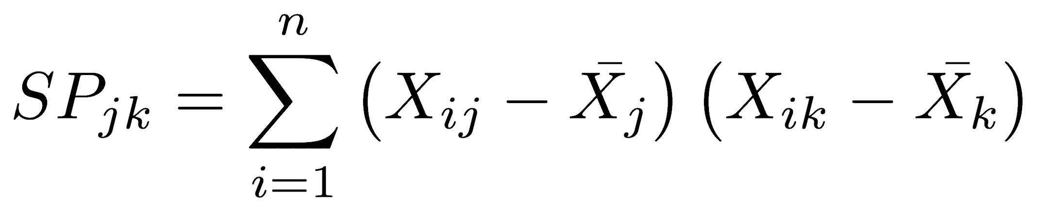
where i is the observation number, n is the total number of observations, j is one variable, and k is the other variable. The sum of products is the deviations from the mean of one variable, multiplied by the deviations from the mean for the other variable, summed over all members of the data series.
The sum of products can also be calculated in a single pass, that is, without first calculating the means:
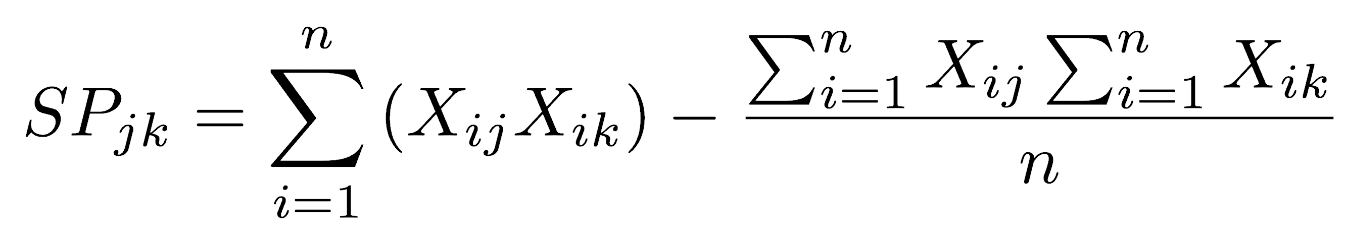
In this formulation, the first term is the uncorrected sum of products, and the second is the correction term. It is “corrected” in the sense that it subtracts the mean from each of the observations. In other words, it is the sum of products relative to the means of each variable, just as we measured the sum of squares relative to the mean.
Covariance is the sum of products divided by the n-1 degrees of freedom. Note the similarity in the formulas for variance and covariance.

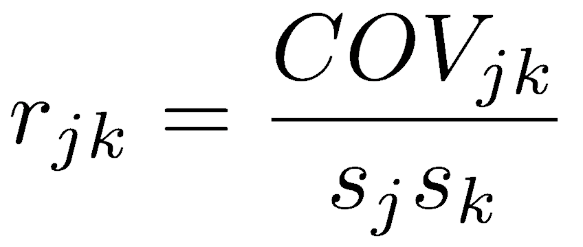
Unlike the sum of squares and variance, which can have only positive values (or zero), the sum of products and covariance can be positive or negative. Covariance has units equal to the product of the units of the two measurements, similar to variance, which has units that are the square of the measurement’s units. Also like variance, covariance is a function of the scale on which the data were measured, which is generally undesirable. Converting covariance into a dimensionless measure produces Pearson’s correlation coefficient.
Pearson’s correlation coefficient
Pearson’s correlation coefficient is also called the product-moment correlation coefficient or just, the correlation coefficient. When someone doesn’t specify the type of correlation coefficient, they usually mean Pearson’s.
To produce a dimensionless correlation measure, we divide covariance by something with the same units, namely the product of the standard deviations of the two variables. This standardizes the joint variation in the two variables by the product of the variation in each variable. The correlation coefficient therefore measures the strength of the relationship between two variables, but it doesn’t depend on the units of those variables.
Pearson’s correlation coefficient varies from -1 (perfect negative linear relationship) to +1 (perfect positive linear relationship). A value of 0 indicates no linear relationship, which occurs when covariance equals zero. If one variable does not vary, one of the standard deviations will be zero, causing the denominator to be zero and making the correlation coefficient undefined.
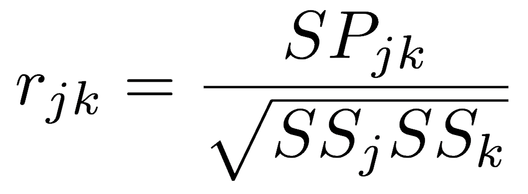
Pearson’s correlation coefficient can alternatively be calculated as the sum of products divided by the square root of the product of the two sums of squares:
The square of Pearson’s correlation coefficient, r2, is one form of a widely reported statistic called the Coefficient of Determination. This coefficient is extremely useful: it measures the proportion of variation explained by a linear relationship between two variables, making it similar to η2 used in ANOVA. As a proportion, r2 is always between zero and one.
Rank (monotonic) correlation
Pearson’s correlation coefficient measures how well a line describes the relationship between two variables, but two variables can have nonlinear relationships that are monotonic. In monotonic relationships, as one variable increases, the other consistently increases or consistently decreases. There are two common choices for measuring the strength of monotonic relationships. Both are non-parametric, and both allow the use of ordinal data, in addition to the interval and ratio data that Pearson’s coefficient requires. Both also range from -1 (perfect negative correlation) to 0 (no correlation) to +1 (perfect positive correlation).
The Spearman’s rank correlation coefficient (ρ, rho) is the more common on the two. Spearman’s coefficient is the Pearson correlation of the ranks of the each variable. In other words, imagine ranking all values of the x variable, assigning 1 to the smallest value, 2 to the next smallest, and so on, doing the same for the y-variable, and then calculating the Pearson correlation of these ranks. When the two variables have a perfect monotonic relationship, the ranks for the two variables would be either identical (a positive correlation) or reversed (a negative correlation).
Kendall’s rank correlation coefficient (τ, tau) is a less commonly used coefficient. Its computation is more complicated than Spearman, but it is based on counting the cases whether pairs of x values are consistently ordered the same as their corresponding pairs of y values.
Kendall is less commonly used than Spearman, and many statistical texts mention only Spearman, so good guidance is scarce. The two metrics tend to produce similar values when the correlation is weak (Sokal and Rohlf 1995). Some have noted that the values of Spearman tends to be larger, sometimes substantially so (Colwell and Gillett 1982), but this seems to be anecdotal. Despite the limited comparative discussions, there are cases where one of the metrics may be more appropriate. Because Spearman places greater weight on dissimilar rankings, whereas Kendall weights all ranks equally, Spearman should be preferred when the validity of similar rankings is uncertain (Sokal and Rohlf 1995). Similarly, Kendall reportedly performs better when there are numerous tied ranks (Legendre and Legendre 1998). Demonstrations of these assertions are hard to find.
Statistical tests
All three metrics can be used simply as a statistic, as a description of the data, and all three are calculated using the cor() function in R. The default method is Pearson, so you need to specify the method argument if you wish to calculate the Spearman or Kendall coefficients.
cor(x, y) # Pearson, by default cor(x, y, method="spearman") cor(x, y, method="kendall")
However, statistical tests should always be used to evaluate these measures. Again, all three use the cor.test() function, and Pearson is the default measure. Spearman and Kendall must be specified through the method argument.
cor.test(x, y) # Pearson, by default cor.test(x, y, method="spearman") cor.test(x, y, method="kendall")
Pearson’s coefficient
We can generate confidence intervals around Pearson’s r and test hypotheses because its distribution is known when some conditions are met. If the data are normally distributed, and if the null hypothesis is that there is zero correlation, Pearson’s correlation coefficient follows a t-distribution, where the standard error of Pearson’s correlation coefficient (sr) is:
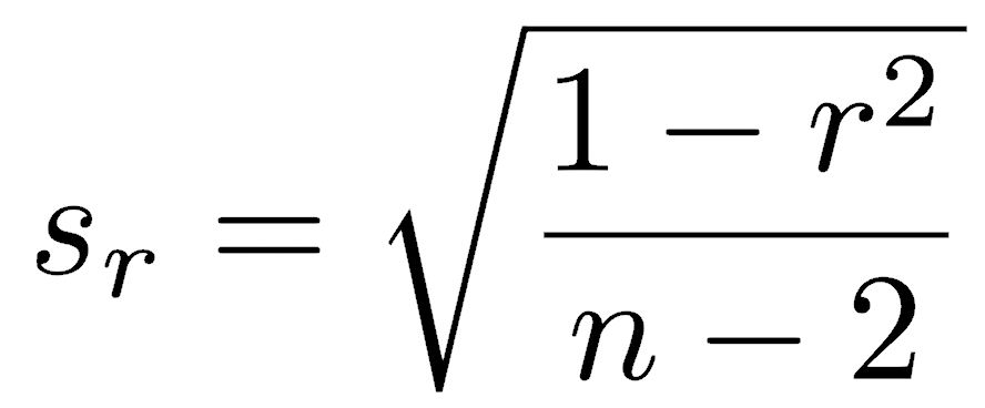
The t-test for Pearson’s r has the standard setup, that is, the statistic minus the null hypothesis for the parameter, divided by the standard error of the statistic:
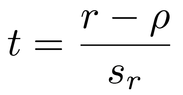
Since the null hypothesis is that the correlation is zero, the ρ term drops out, and the t-statistic is simply Pearson’s correlation coefficient divided by its standard error. The t-test of Pearson’s correlation coefficient has n-2 degrees of freedom because the population variance is estimated for two variables instead of one.
The t-tests of Pearson’s r therefore has four assumptions. First, the data must be interval or ratio (also called measurement variables). Second, the data must be randomly sampled from the population. Third, the variables must follow a normal distribution. Last, the test assumes that the null hypothesis is that the correlation is zero.
Like other parametric tests in R, the output provides an estimate of the statistic (the correlation coefficient), a confidence interval on the statistic, and a p-value (corresponding to a null hypothesis of zero correlation). Confidence levels other than 95% can be set with the conf.level argument, and one-sided tests can be specified with the alternative argument. As always, you must have external reasons for specifying a one-sided test: you cannot observe the correlation and decide on a one-sided test based on that observation.
If your data are not normally distributed, confidence intervals must be calculated through other methods, such as the bootstrap and jackknife. Alternatively, consider one of the methods suggested by Bishara and Hittner (2019).
Spearman and Kendall coefficients
Statistical tests for both of these metrics assume only that the two variables are random samples of their populations. The data may be ordinal, interval, or ratio. Tests for both provide a p-value, but no confidence interval. If you want to generate a confidence interval, perform a bootstrap or jackknife. This post by Thom Baguley suggests other ways to calculate a confidence interval.
If you have nominal data and want to measure the association between variables, the χ2 (chi-squared) and G-test are common approaches.
Rank correlation is less affected by outliers than Pearson
Rank correlation methods are generally preferred when data have outliers because of their strong effects on the Pearson correlation coefficient. For example, one outlier (in red, upper right) is added to the data below. Notice how much the outlier increases the Pearson correlation compared with the Spearman correlation.
x <- rnorm(10) y <- rnorm(10) plot(x, y, pch=16, xlim=c(-3,5), ylim=c(-3,5)) cor(x, y) # -0.49 cor(x, y, method="spearman") # -0.21 # Add one outlier x <- c(x, 5) y <- c(y, 5) points(x[11], y[11], pch=16, col="red") cor(x, y) # 0.76 cor(x, y, method="spearman") # 0.09
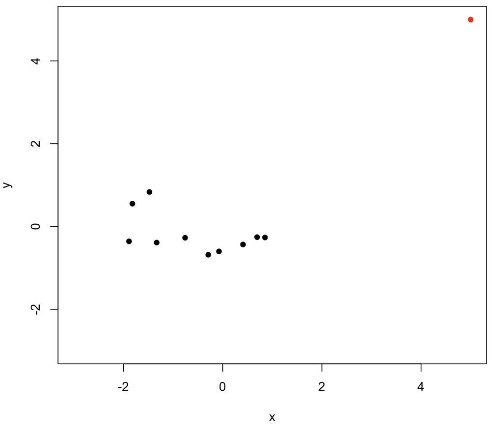
The insensitivity of Spearman to outliers comes from its use of ranks: no matter how large the largest value becomes, its rank never changes, and it’s still just the highest-ranked point. As always, plot your data first to know if outliers are an issue.
Some relationships can be linearized
Although Pearson’s correlation measures linear correlations, consider a data transformation before resorting to a rank correlation measure when the relationship is nonlinear. For example, consider the following plot, which shows an exponential relationship.
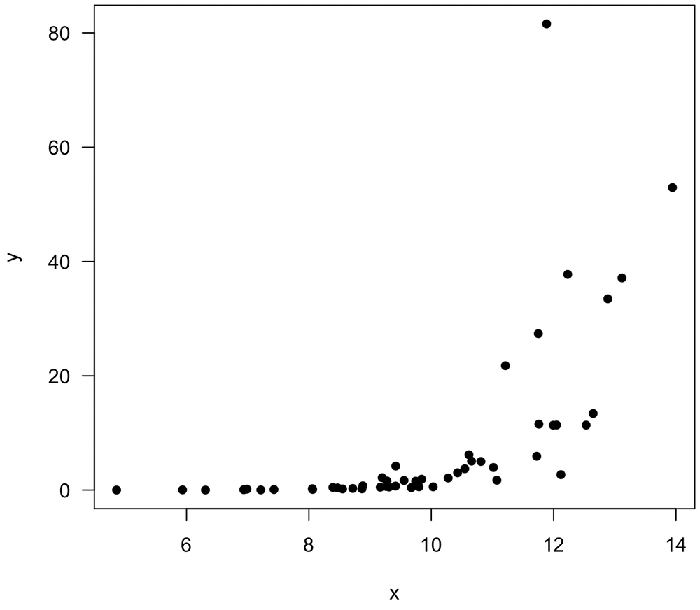
A log transformation of the y variable linearizes the relationship, such that Pearson’s correlation could be calculate for x and log(y).
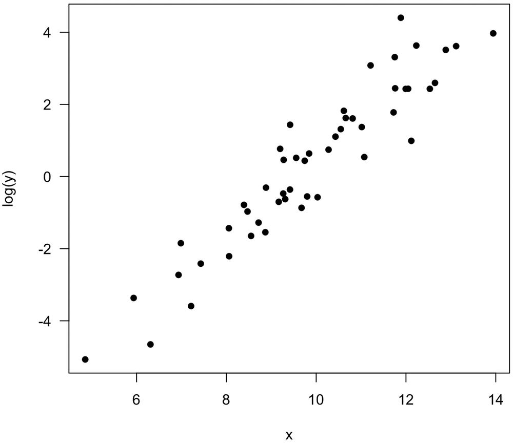
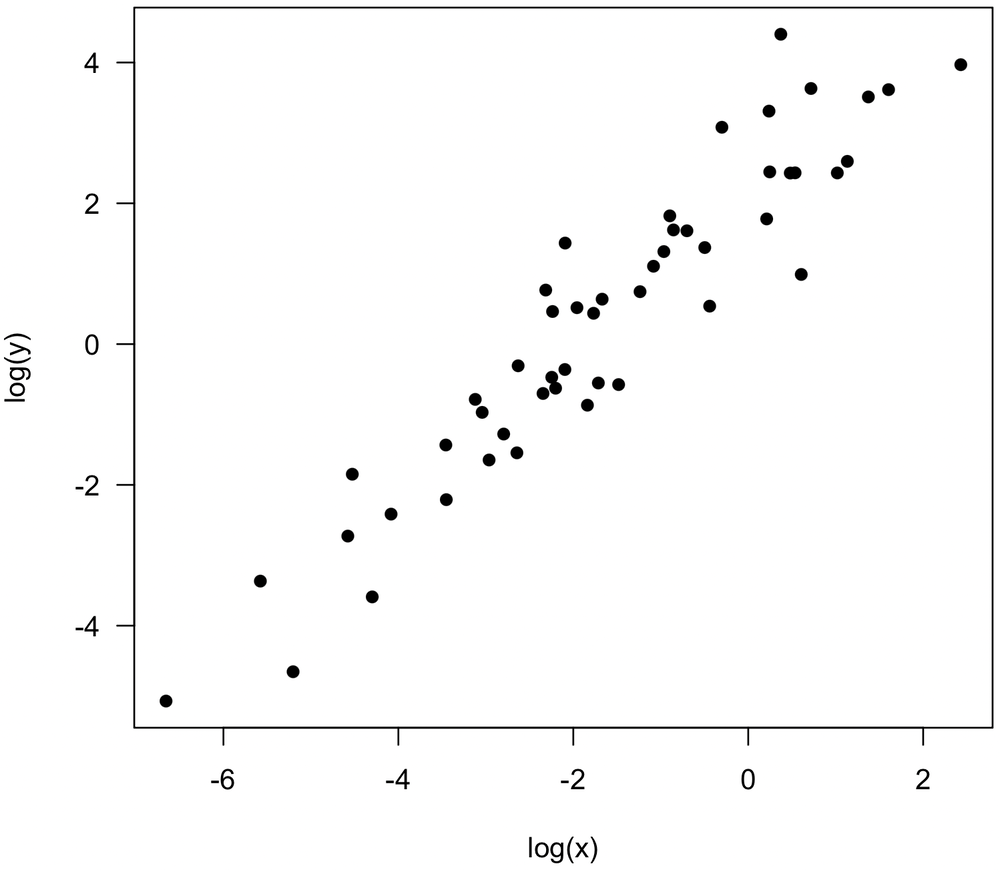
Similarly, consider this noisy plot, which suggests a weak positive relationship between x and y.

Log transformations of both variables reveal a stronger relationship, and Pearson’s correlation should be calculated on log(x) and log(y). In both examples, it suggests that at least one variable is more properly measured on a logarithmic scale than a linear one, a common situation in the natural sciences.
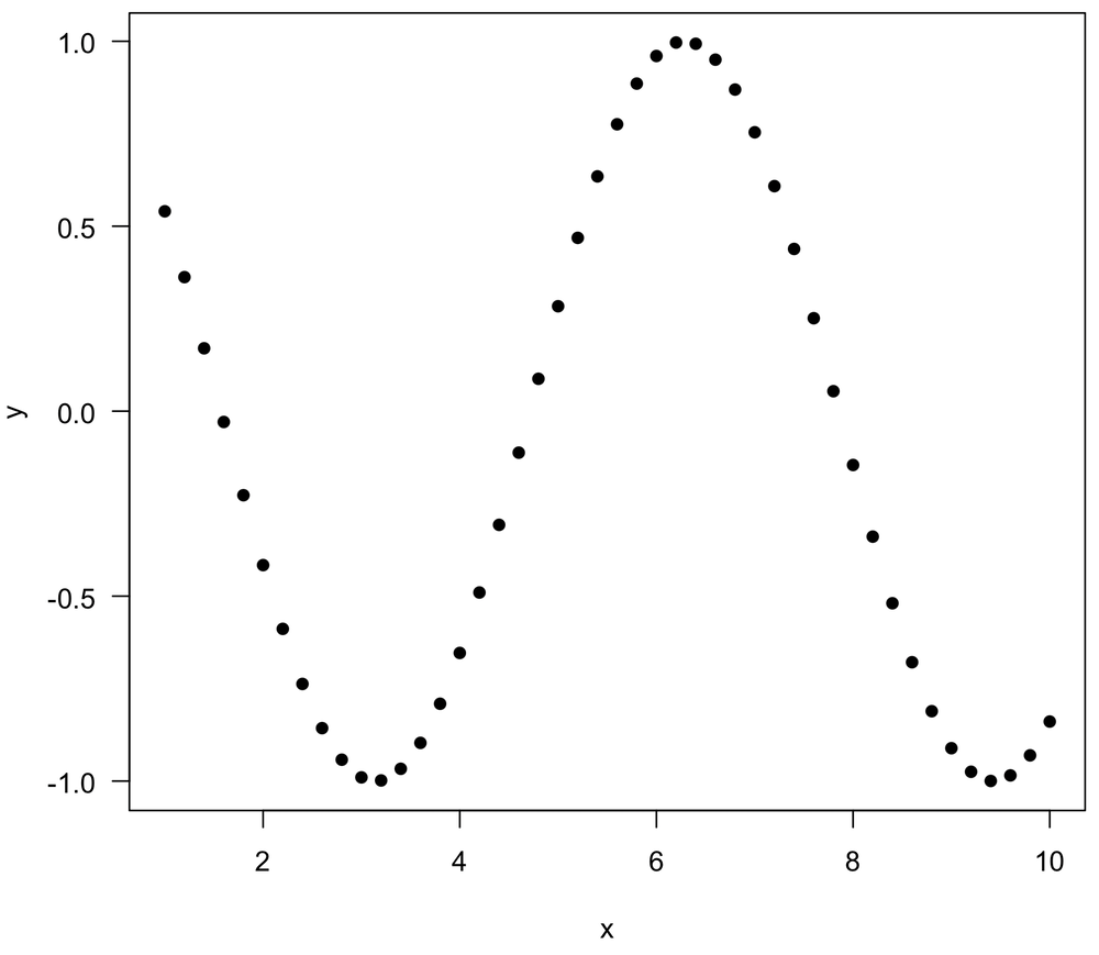
Some relationships are neither linear or monotonic
Two variables can have strong relationships that are neither linear nor monotonic, such as a sine wave. In these cases, all correlation coefficients may be near zero, even though a very simple relationship may underlie the data. Always plot your data first to understand what the relationship looks like, and always use the appropriate correlation measure to describe your data. For this example, the coefficient of determination (discussed in the regression lectures) is a good measure of the strength of the relationship.
x <- seq(1, 10, by=0.2) y <- cos(x) plot(x, y, las=1, pch=16) cor(x, y, method="pearson") # -0.04 cor(x, y, method="spearman") # -0.07
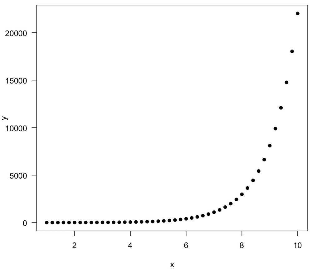
Pearson and Spearman correlations can be quite different
Pearson and Spearman (and Kendall) measure different types of relationships: linear vs. monotonic. A relationship can be monotonic and non-linear, and as a result, it may have a stronger Spearman correlation than a Pearson correlation. An example demonstrates this:
> x <- seq(1, 10, by=0.2) > y <- exp(x) > plot(x, y, las=1, pch=16) > cor(x, y, method="pearson") [1] 0.71554 > cor(x, y, method="spearman") [1] 1
Time series commonly have spuriously high correlations
Random walks commonly show a strong and statistically significant correlation with one another. As you might expect, increasing the time series length (that is, sample size, n) causes the correlation to have even greater statistical significance, that is, a lower p-value. As a result, two unrelated time series are often have a statistically significant and potentially large correlation. This behavior often arises when the two variables are correlated to a third variable, such as time
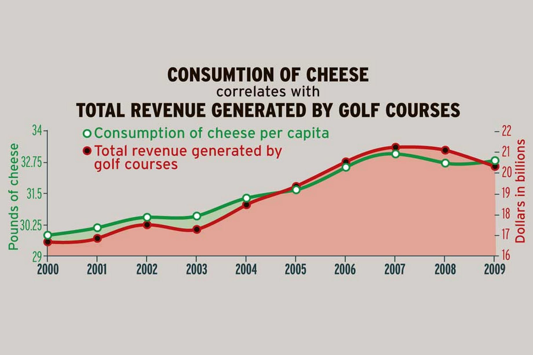
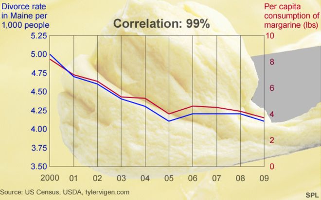
For example, the number of ministers and the number of alcoholics are positively correlated through the 1900’s. The number of each largely reflects the growing population during that time, so the two display a correlation, even though there is no direct link between the two. There are plenty of other examples.
The spurious correlation of two random walks is easily simulated by taking the cumulative sum (also called the running sum) of two sets of random numbers:
x <- cumsum(rnorm(25)) y <- cumsum(rnorm(25)) cor(x, y)
Because random walks are unrelated, you might expect a correlation test of random walks to produce a statistically significant result at a rate equal to α (e.g., 5%), that is that 5% of random walks would have a statistically significant correlation. This is known as the Type I error rate, the proportion of times that a true null hypothesis (here, no correlation) is rejected. Statistically significant correlations of random walks are far more common than that, meaning that the type I error ratencan be much larger than α, the significance level. You can see this by running the following code several times; p-values less than 0.05 occur far more frequently than the expected 1 out of 20 times.
x <- cumsum(rnorm(25)) y <- cumsum(rnorm(25)) cor.test(x, y)$p.value
A spurious correlation is a problem not only for time series but also for spatially correlated data.
You might think that you could address the problem of spurious correlation by collecting more data, but this worsens the problem because increasing the sample size will lower the p-value.
Spurious correlation can be solved by differencing the data, that is, calculating the change from one observation to the next, which reduces by one the size of the data set. Differencing the data removes the time (or spatial) correlation, removing the dependence of a value on the preceding value. Differenced data will not display spurious correlation because the trends are removed. Use the diff() function to calculate your differences quickly.
xdiff <- diff(x) ydiff <- diff(y) cor(xdiff, ydiff)
Whenever you encounter someone trying to correlate time series or spatial series, ask if the data were differenced. If they were not, be skeptical of any non-zero correlation and any claims of statistical significance, especially when the sample size is large.
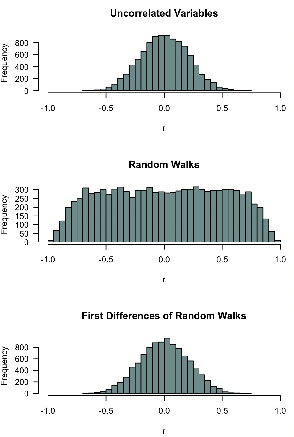
Here is a simulation that illustrates the problem of spurious time-series correlation. Each plot shows 10,000 random simulations of the correlation coefficient of two data series. The upper plot shows the results for two uncorrelated variables, the middle plot shows two random walks (time series), and the bottom plot shows two differenced random walks (time series). Note how commonly two random walks can produce strong negative or positive correlations, and note how differencing returns the expectation to that of two uncorrelated variables.
par(mfrow=c(3,1))
trials <- 10000
n <- 25
r <- replicate(trials,
cor(rnorm(n), rnorm(n)))
hist(r, xlim=c(-1, 1), breaks=50, col="paleturquoise4", las=1,
main="Uncorrelated Variables")
r <- replicate(trials,
cor(cumsum(rnorm(n)), cumsum(rnorm(n))))
hist(r, xlim=c(-1, 1), breaks=50, col="paleturquoise4", las=1,
main="Random Walks")
r <- replicate(trials,
cor(diff(cumsum(rnorm(n))), diff(cumsum(rnorm(n)))))
hist(r, xlim=c(-1, 1), breaks=50, col="paleturquoise4", las=1,
main="First Differences of Random Walks")
References
Colwell, D.J., and J.R. Gillett. 1982. Spearman versus Kendall. The Mathematical Gazette 66:307–309.
Legendre, P., and L. Legendre. 1998. Numerical Ecology, 2nd English edition. Developments in Environmental Modeling 20. Elsevier, Amsterdam, 853 p.
Sokal, R.R., and F.J. Rohlf. 1995. Biometry, 3rd edition. Freeman, New York, 887 p.
