Generalized Additive Models
The regression models we have considered so far — linear models with lm(), nonlinear models with nlm(), and generalized linear models with glm() — all require that we have a preconceived notion of the form of the model to be fit to the data. Sometimes we don’t, and generalized additive models (GAM) provide a way to fit a function to the data along with an uncertainty envelope. Although they generally do not provide a function with coefficients and their uncertainties, they do provide a means of prediction and significance tests based on p-values. GAMs are especially useful for exploratory data analysis and for fitting functions to patterns that do not conform to simple mathematical models.
GAMs are most commonly implemented with the gam() function in the mgcv package. At their simplest, GAMs use smoother functions specified by using s() in the model formula:
library(mgcv) model <- gam(y ~ s(x))
Fitting a GAM is demonstrated here with a simulated data set of the body mass and home range of species.
ecology <- read.table("massRange.csv", header=TRUE, sep=",") attach(ecology) logRange <- log10(ecolRange) logMass <- log10(bodyMass) model <- gam(logRange ~ s(logMass)) plot(model, residuals=TRUE, pch=16, rug=FALSE, las=1, cex=0.5, xlab="log(mass, kg)", ylab="log(range, acres x 1000)")
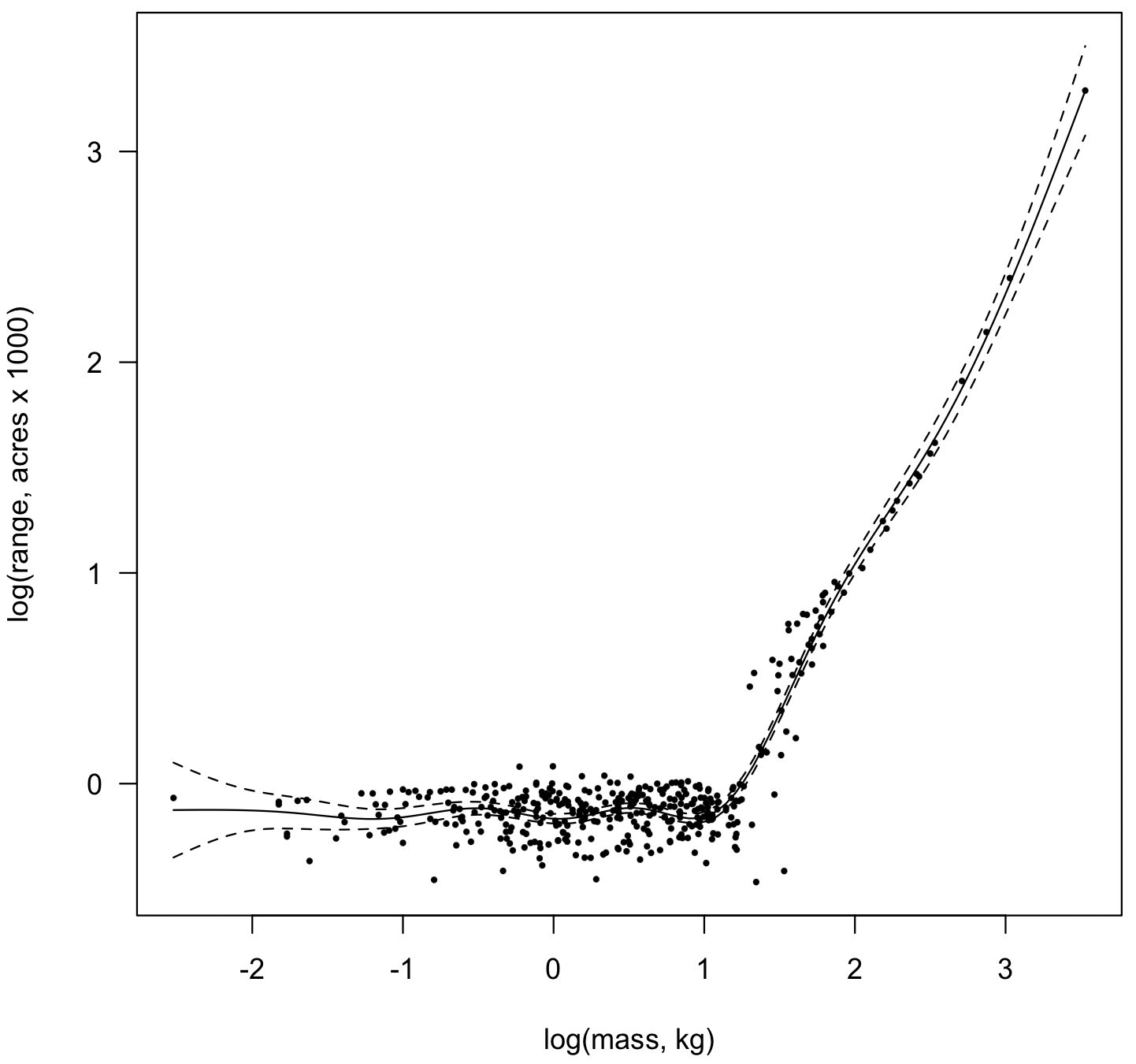
The model reveals a dog-leg pattern in the relationship of home range of species as a function of body size. Below about 20 kg, home range has a relatively constant size, but increases more or less linearly above 20 kg.
Other applications
A variety of smoothing functions and parameters are available; see the help page for details. Generalized additive models can be simplified and compared, much as described for multiple regression using lm(). Alternative error models and link functions can also be specified as they are for generalized linear models through the glm() function.
For example, a GAM could be fitted to binary data by specifying the family=binomial, as would be done with glm(). In this made-up example, extinction is modeled as a function of body mass.
event <- read.table("bodyMassExtinction.csv", header=TRUE, sep=",") attach(event) model <- gam(becameExtinct ~ s(bodyMass), family=binomial) plot(model, residuals=TRUE, rug=FALSE, pch=16, cex=0.5) summary(model)
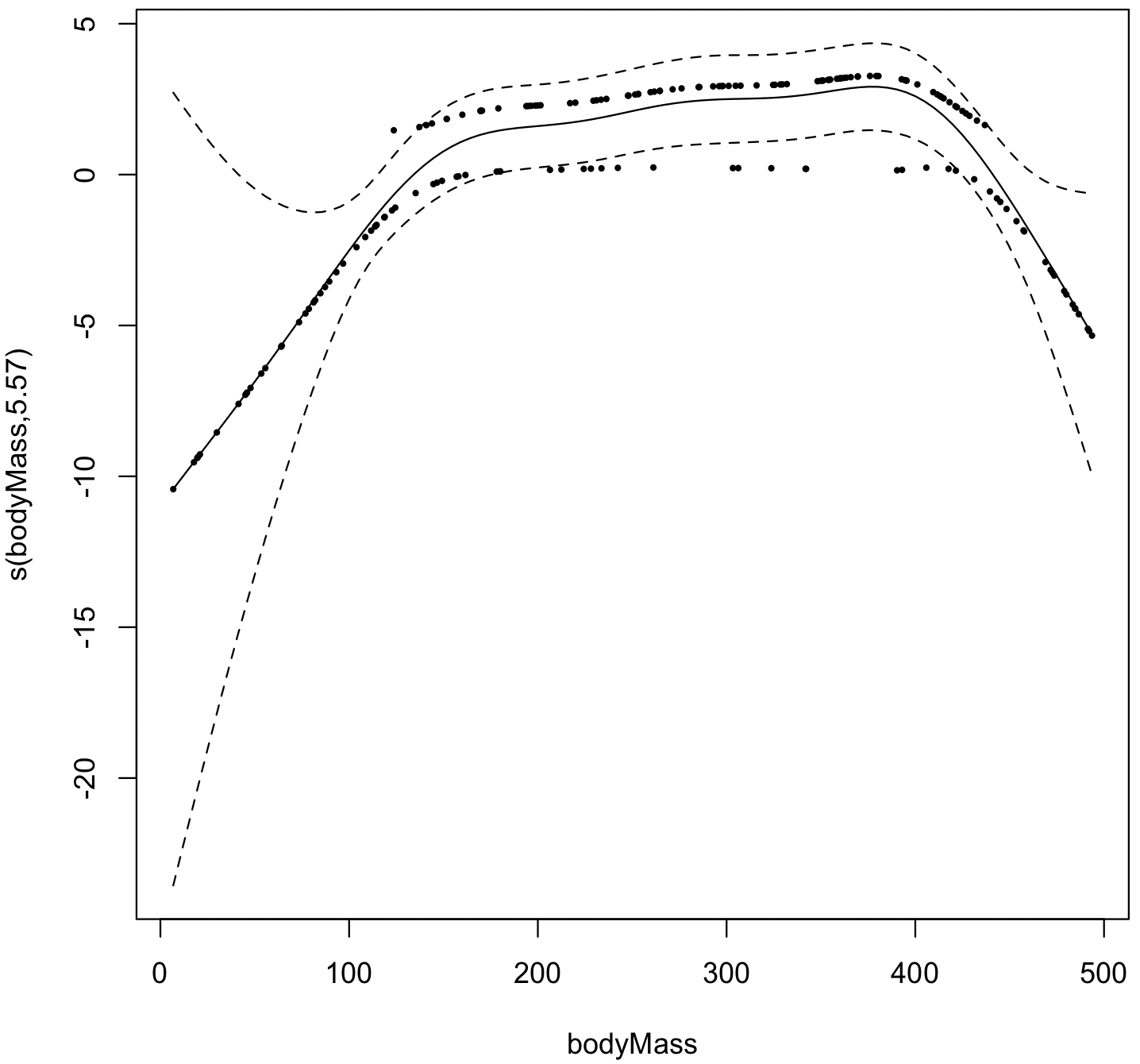
The model indicates that extinction was primarily limited to species of intermediate body size.
References
Crawley, M. J. 2013, The R Book, 2nd edition. Wiley, Chichester.
