p-values and Confidence Intervals
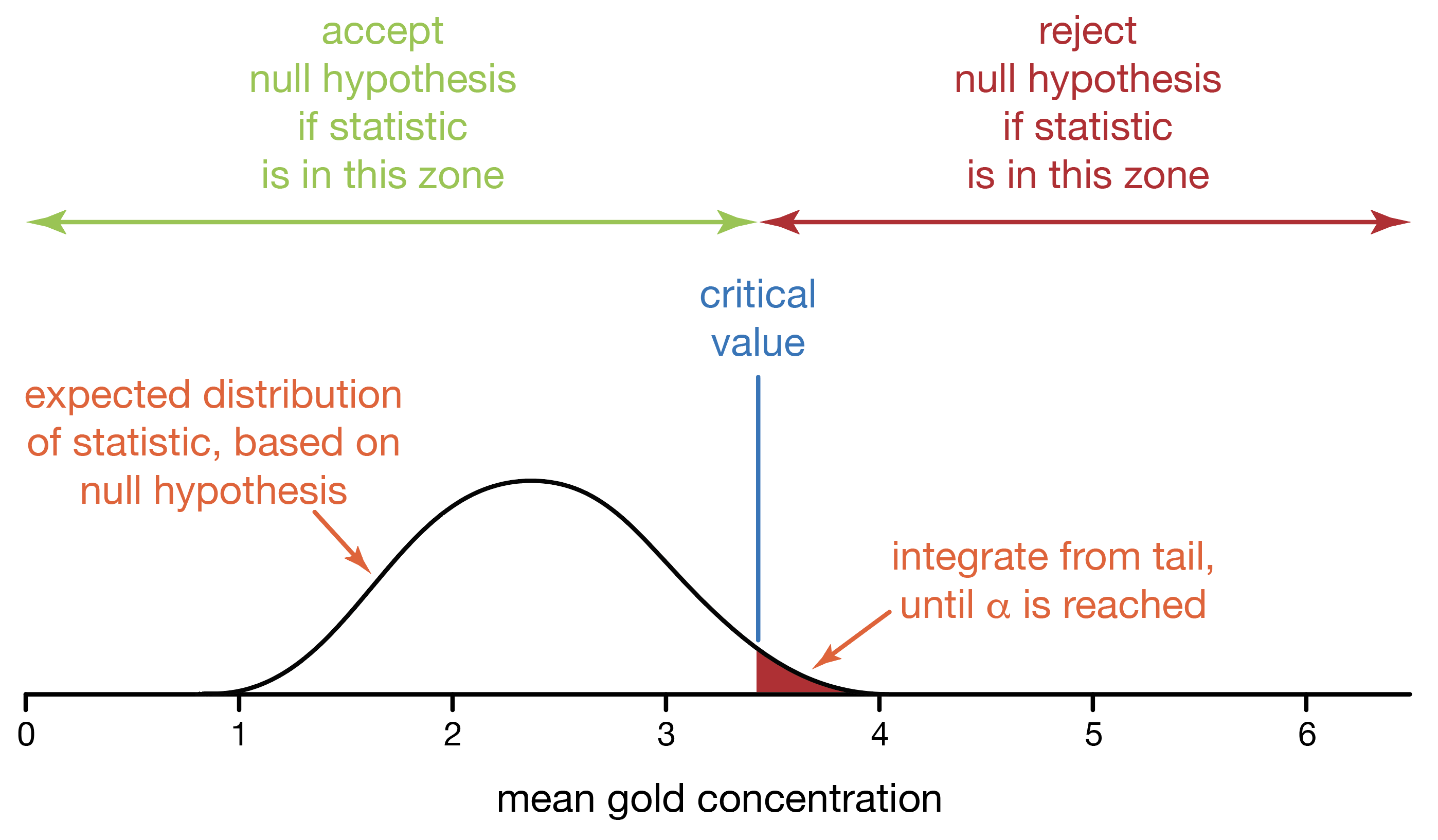
In the critical-value approach to statistical testing, we (1) state a null and alternative hypothesis, (2) generate a distribution of outcomes based on the null hypothesis, (3) choose a significance value, (4) find our critical value(s), (5) measure our statistic, and finally, (6) decide whether to accept or reject the null hypothesis.
When we report our decision, there is no simple way to convey how convincingly we made our decision. Was our null hypothesis clearly rejected or accepted, or was it a borderline case? Even if the observed and critical values seem close, we would have to know the shape of the distribution to tell if the decision was borderline or not. The all-or-nothing, accept-or-reject approach of critical values proides an incomplete picture.
p-values: a second approach to statistics
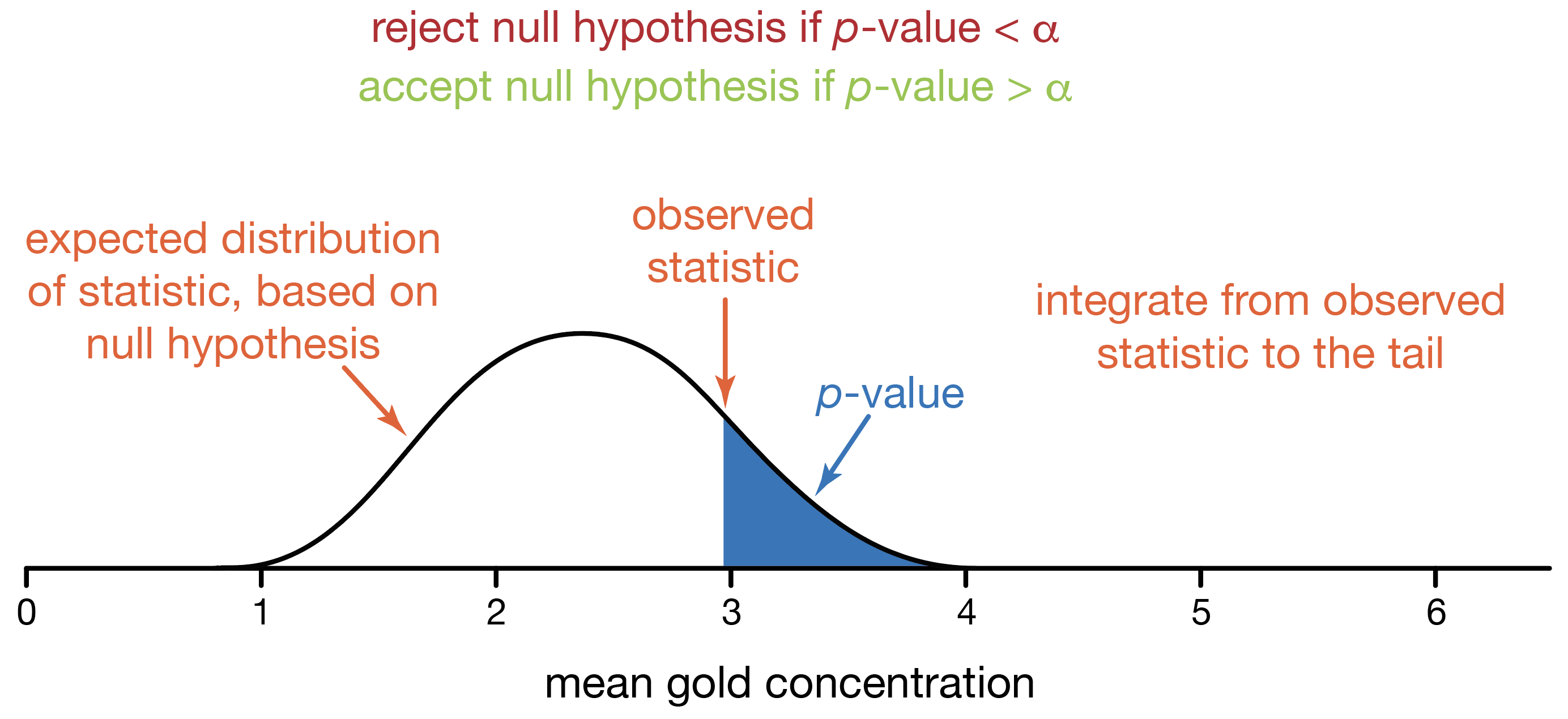
Another approach, developed by Ronald Fisher (of F-test, maximum likelihood, genetics, and evolutionary biology fame), lets us show how well-supported our decision is. We again start with a distribution of outcomes based on the null hypothesis. Instead of finding a critical value, we use our observed statistic and calculate the probability of observing it or a value even more extreme. This probability is called a p-value. A p-value is the probability of observing a statistic or one more extreme if the null hypothesis is true. Memorize this definition.
We use the p-value and α (significance) to make a decision about the null hypothesis. If the p-value is less than α, we conclude that our statistic has such a low probability of being observed when the null hypothesis is true that we should reject our null hypothesis. If our p-value is greater than α, we accept our null hypothesis because our p-value tells us that our observed statistic is a probable result when the null hypothesis is true.
Finding a p-value is the reverse of finding a critical value. When you find a critical value, you start with a probability (α, significance) and integrate the probability distribution starting from one or both tails until you equal that probability. The critical value(s) correspond to those cutoff values of the statistic. With a p-value, you start with the observed statistic, and integrate the probability distribution from the statistic towards the tail. That cumulative probability from your statistic to the tail is the p-value.
P-values improve on the critical-value approach to statistics. We can still decide to accept or reject the null hypothesis, just as we did in the critical-value approach. Moreover, this will result in the same decision as one based on critical values. We can also report the p-value, which directly reports the probability of observing what we did (or a value more extreme) if the null hypothesis is true. With this, anyone can judge whether the null hypothesis can be convincingly rejected or accepted, and whether this is a borderline or clear-cut decision. For example, a tiny p-value says we have an extremely unlikely result if the null is true, whereas a large p-value shows that our observations are consistent with the null hypothesis. P-values convey more information than the critical-value approach, so scientists today primarily use the p-value approach.
Three quantities control the size of a p-value. First, it partly reflects effect size, with larger effect sizes producing smaller p-values. Effect size is what is being investigated, for example, a correlation coefficient, a difference in means, a ratio of variances, a slope, etc. Effect sizes are not under our control. Second, the size of a p-value is controlled by sample size, and larger sample sizes generate smaller p-values. Third, it reflects the variation inherent in what is being studied: greater variation produces larger p-values.
Confidence intervals: a third alternative
The critical-value and p-value approaches test only a single null hypothesis, most commonly that a parameter (mean, correlation coefficient, etc.) is zero. Alternatively, you might want to know all the hypotheses that are consistent or inconsistent with the data, not just the null hypothesis. Even more, sometimes it is unclear what the null hypothesis is, and this is a problem: without a null hypothesis, you cannot generate the probability distribution needed to calculate a critical value or a p-value.
There is an alternative. Imagine being able to test every possible hypothesis and identify those that are consistent with the data and those that are not. Confidence intervals do just that. Although testing all possible hypotheses sounds laborious, calculating confidence intervals is usually as easy as calculating a p-value.
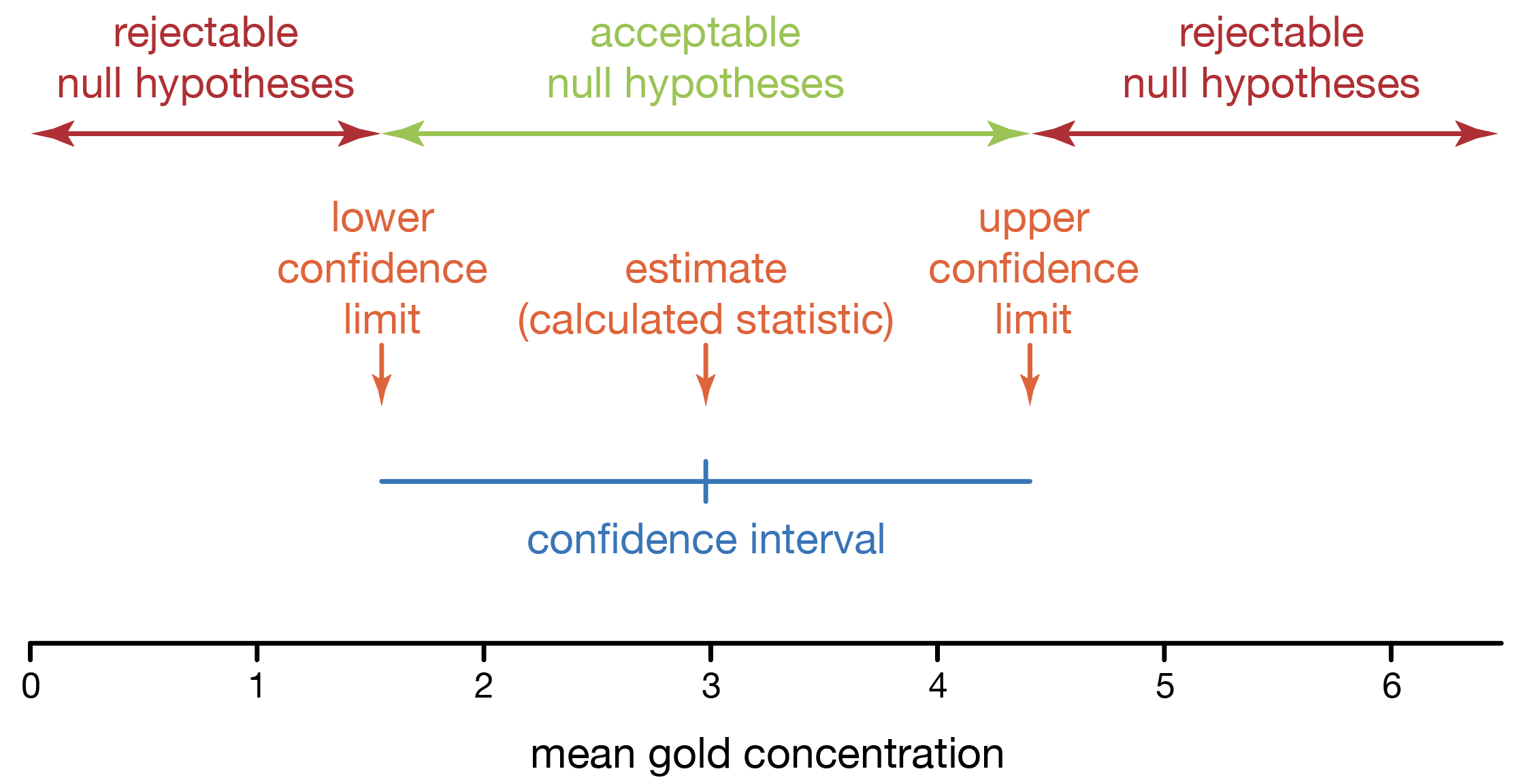
Unlike the critical-value approach and p-values, confidence intervals are calculated from the data, not from a probability distribution based on the null hypothesis. If some assumptions are made about the parent distribution underlying the data, it is possible to construct the distribution of any statistic from our data. From this distribution, we can use our significance level (α) to establish the limits (called confidence limits) of what parameter values would be considered consistent with the data. We use these limits to define a confidence interval of parameter values consistent with the data; this region always includes and is often centered on the observed statistic. A confidence interval is the entire region, and the confidence limits mark the endpoints of the confidence interval.
A confidence interval is the set of all hypotheses that are consistent with the data. Memorize this definition. Another way to say this is that a confidence interval is the set of all acceptable null hypotheses. In other words, you would accept any hypothesis within the confidence interval, including the confidence limits (the endpoints of the confidence interval). You reject any hypothesis that lies beyond the confidence limits.
As always, acceptance and rejection do not mean that the hypothesis is true or false. If you accept the hypothesis, you are saying it is one plausible explanation for the data. You are also acknowledging that there may be other plausible hypotheses. When you reject a hypothesis, you are saying that the data would be unlikely if the hypothesis were true.
Confidence intervals are more informative than the critical-value and p-value approaches in that they convey an estimate of a parameter and an uncertainty in that estimate. The statistic we calculate from our data (for example, the mean or the correlation coefficient) becomes our estimate for the parameter. The confidence interval describes our uncertainty in that estimate. This is far more informative than the critical-value and p-value approaches, and confidence intervals should be your standard practice. Confidence intervals rightly shift our attention from a probability (the p-value) to what we are measuring and our uncertainty in it.
Confidence limits are generally phrased as a value (the statistic, our best estimate of a parameter) plus or minus another value (the uncertainty). For example, 13.3 ± 1.7 describes a confidence interval of 11.6 to 15.0. A large confidence interval conveys large uncertainty in your estimate of the parameter, and a small interval indicates a high degree of certainty. Confidence intervals are always reported with the confidence level, which reflects the significance level. For example, 95% confidence limits correspond to a significance level (α) of 0.05.
Confidence intervals have a specific interpretation. If your confidence is 95%, approximately 95% of the confidence intervals you construct in your lifetime will contain the population parameter. Confidence intervals do not mean that there is a 95% chance that you have bracketed the population mean in a particular case, and this misconception is widespread. The reason why confidence intervals cannot mean this is that no probability is involved once the confidence interval has been calculated. Once the confidence interval and population parameter both exist, there is no element of chance: the parameter either lies within the confidence interval, or it doesn’t. Without chance, there is no probability.
Three quantities control the size of a confidence interval. First, sample size matters, and larger sample sizes generate tighter confidence intervals, indicating less uncertainty in your estimate of the parameter. As always, having larger sample sizes is good. Second, the variation in the data matters: greater variation produces broader confidence intervals. In other words, as the variation in the data becomes larger, so does the uncertainty in any parameter estimate. Third, your chosen confidence level (1-α) affects the size of confidence intervals: larger confidence levels create broaden confidence intervals. This may seem counterintuitive, but one way to think about this is that as your confidence increases, your confidence intervals become more likely to bracket the population mean, which means they must get larger.
Here is the handout and demonstration R code for today’s lecture.
Reading
Be sure to read this section from Biometry (Sokal and Rohlf, 1995) on Type I and Type II errors. Although Sokal and Rohlf illustrate these concepts with a specific statistical test, you should focus on the principles we discussed in class, not on the particulars of the test they use.
References
Sokal, R. R., and Rohlf, F. J., 1995, Biometry: New York, W.H. Freeman and Company, 887 p.
