Box-and-whisker plots
8 June 2025
Box-and-whisker plots are an effective way of summarizing data and visualizing their distribution. Although box-and-whisker plots typically do not show the data points, they do display the median and the interquartile range, and they can be useful for identifying potential outliers.
The basics
Boxplots are easily generated in R with the boxplot() function, automatically included as part of the {graphics} package. For this demonstration, we’ll simulate the data as weights of 100 beetles that follow a log-normal distribution.
weight <- rlnorm(100) boxplot(weight)
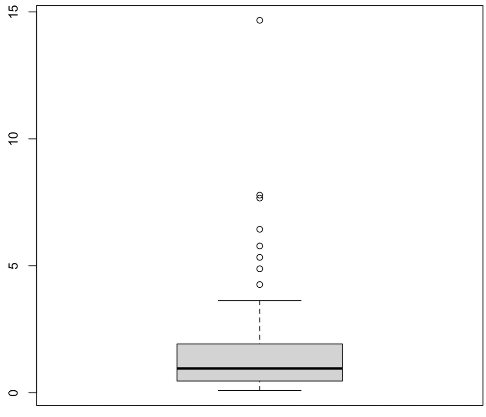
Simple customizations
The default plot has several issues. There is far too much white space, the axes are not labeled, and the y-axis vales are turned on their side. We can resize the plot window to eliminate the excess white space, turn the plot horizontal by setting horizontal=TRUE, and add the axis label with xlab.
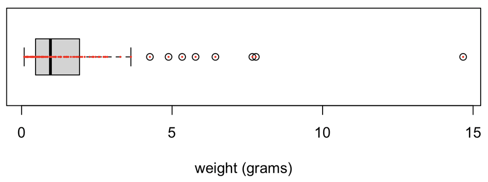
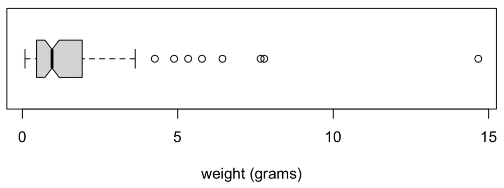
boxplot(weight, horizontal=TRUE, xlab="weight (grams)")

This is a much more space-efficient way of showing this plot.
Adding the data
We can also add the points to the plot with a call to points(). I’ve made them filled circles (pch=16) that are small (cex=0.3) and red (col="red").
points(weight, rep(1, length(weight)), pch=16, cex=0.3, col="red")
What is shown
Adding the points in this demonstration helps understand what the box-and-whiskers plot depicts.
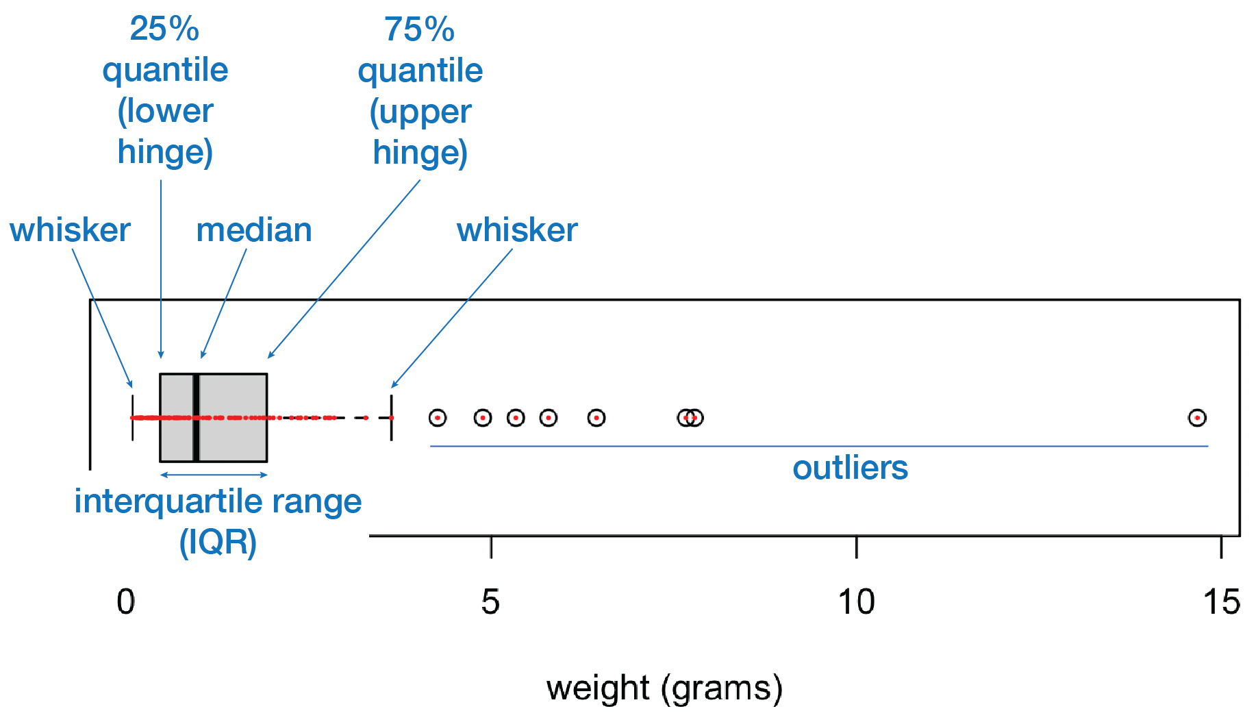
The vertical black bar is the median, also called the 50% quantile, meaning that 50% of the values are smaller. The box is bounded by the 25% quantile and the 75% quantile, which are called the lower and upper hinges (also known as quartiles). As the median divides the data equally, you can think of the lower hinge as the median of the values that are smaller than the overall median, with the upper hinge being the median of the values to the right of (larger than) the overall median. The width of the box, that is, the distance between the two hinges, is called the interquartile range or IQR.
Two whiskers are added that encompass most of the remaining values. The whiskers can be placed in several ways. The default in R is to place them at the last value that falls within 1.5 times the interquartile range above or below the median. On this plot, the smallest data point is within 1.5 * IQR left of the median, so the left whisker corresponds to the smallest value in the data. Eight data points on the right side lie beyond 1.5 * IQR above the median, so the whisker is drawn at the last data point that lies within this range.
The 1.5 multiplier is arbitrary. Sometimes the whiskers are drawn at the largest and smallest values; this can be done by adding range=0 to the boxplot() call. If you wanted the multiplier to be 2.0, you would set range=2. Given the number of possibilities, always specify how the whiskers are drawn in your methods section.
Outliers
Points that lie beyond the whiskers are considered outliers. As always, outliers are not necessarily a problem in the data. In this example, the numerous outliers on the right side of the distribution, with none on the left, suggest that the data are right-skewed. This is underscored by the median lying towards the left of the interquartile range and by the right whisker being longer than the left. All of this suggests that a data transformation is necessary.
A log transformation of the data solves these issues (unsurprising, since we started with a log-normal distribution!).
boxplot(log(weight), horizontal=TRUE, xlab="log(weight) (grams)") points(log(weight), rep(1, length(weight)), pch=16, cex=0.3, col="red")
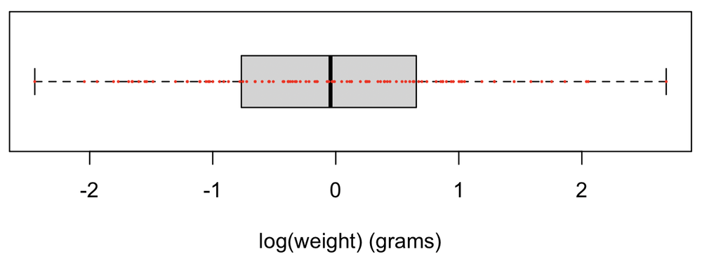
Now, the box-and-whiskers plot is symmetrical and there are no outliers. Even so, it is not unusual for a point or two to lie outside the whiskers, and for that to not be a concern.
The notch
Box-and-whiskers plots often include a notch or waist at the median. The width of the notch is a measure of the uncertainty in the median; see McGill et al. 1978 for ways the notch width might be calculated. Given the various ways in which notches may be calculated, always state in your methods how notches were drawn. Notches are most useful when multiple box plots need to be compared. Notches are added by including notch=TRUE in the call to boxplot().
boxplot(weight, notch=TRUE, horizontal=TRUE, xlab="weight (grams)")
Multiple groups
Box-and-whisker plots for multiple groups can be easily shown on one plot. This example uses the InsectSprays data included with R, where count is a vector reporting the number of insects and spray is factor indicating which bug spray was used. Instead of calling boxplot() on a single vector, a model formula is used, the same as it would be for regression. Here, count is a function of spray. By default, bar plots are shown vertically, but they could be flipped to horizontal as described above (i.e., adding horizontal=TRUE to the boxplot() call).
boxplot(count~spray, data=InsectSprays, col="lightgray")
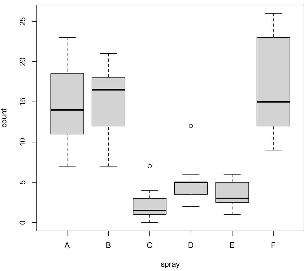
Sprays C, D, and E have markedly smaller insect counts than sprays A, B, and E. One might wonder if the medians within each of these two groups are different, so notches should be added.
boxplot(count~spray, data=InsectSprays, notch=TRUE, col="lightgray")
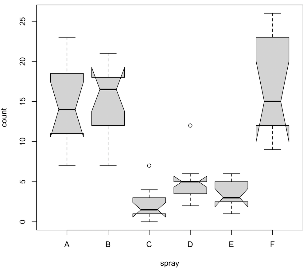
Many of these notches look strange. For example, look at spray F. The upper part of the notch lies within the box (i.e., is smaller than the 75% quantile), but the lower part of the notch extends beyond the box (i.e., is smaller than the 25% quantile). Although R will give you a warning when this happens, it is not a problem, as the box expresses the interquartile range and the notch expresses the uncertainty in the median; the box does not have to be larger than this uncertainty.
Despite the initially odd appearance, the non-overlapping notches of sprays C, D, and E show that their medians are different. The overlapping notches of A, B, and E indicate that their medians are indistinguishable.
Indicating sample size
Because the size of the notch is usually related to sample size (more data means less uncertainty, so a narrower notch width), it can be helpful to scale the widths of the boxes to sample size. This can be done by adding varwidth=TRUE to the boxplot() call, which scales the width of the box by the square root of sample size. This is not done for the insect spray data, as these data have a balanced design: the sample size in all groups is equal.
Using box plots
Use box plots whenever you need to summarize how your data are distributed: they are effective, just like histograms and strip charts. They are especially worthwhile when you need to characterize the median in one or more groups.
Remember to report how the whiskers were calculated, and if you use them, how notches were calculated.
References
McGill, R., J.W. Tukey, and W.A. Larsen. 1978. Variations of box plots. The American Statistician 32:12–16.
