Central Limit Theorem
6 October 2025
The central limit theorem states that the distribution of sample means converges on a normal distribution as the sample size grows, regardless of the shape of the parent distribution. On its face, it suggests that t-tests can be used on any parent distribution, provided that the sample size is large enough. Some authors (including me until recently) argue that this convergence occurs for non-normal distributions at relatively small sample sizes, such that one does not need to be concerned with the shape of the parent distribution except at small sample sizes. Other authors argue that the t-test assumes that the data follow a normal distribution and should not be applied to other distributions.
One way to evaluate these conflicting arguments is to simulate performing a t-test on data drawn from different distributions and measure the type I error rate, that is, the proportion of times that the null hypothesis is rejected. For a given significance level (e.g., α=.05), a statistical test should produce a matching type I error rate. If the assumptions of the test are not upheld, the test is likely to cause the null hypothesis to be rejected more often than the significance level, that is, it is likely to have a type I error rate that is larger than the significance level.
This is easy to evaluate in simulations because the data can be generated from a particular distribution, so the null hypothesis is known to be true. A large p-value (one greater than the significance level) will lead to the correct decision of accepting the null hypothesis. A small p-value (i.e., less than alpha) will lead to rejecting the null hypothesis, an incorrect decision called a Type I error.
I explored the type I error rate for several parent distributions to evaluate how large the sample size must be for the type I error rate to match the significance level. I was surprised by the results.
Experimental design
These numerical experiments use a bootstrap, where the same process is repeated many times. The process here is to create a sample of a given size from a known distribution, perform a t-test, and extract the p-value. This is repeated many times, and I calculate the fraction of times in which the p-value is less than 0.05, the significance level in all my experiments. This fraction is the type I error rate. I perform this same procedure at a range of sample sizes from 5 to 200, then plot the type I error rate vs. sample size.
I ran four experiments: a normal distribution, an exponential distribution, a lognormal distribution, and a lognormal distribution followed by a log transformation. The last of these should, and did, produce the same result as a normal distribution.
The core function that is repeated looks like this:
oneTtest <- function(n, FUN, null) { x <- FUN(n) t.test(x, mu=null, conf.level=0.95)$p.value }
The function takes three arguments: sample size ( n ), the function that will generate the random numbers ( FUN ), and the null hypothesis for that distribution ( null ). The function returns the p-value for a t-test of that null hypothesis.
Two aspects of the design merit comment. First, I performed a 100,000-iteration bootstrap, that is, I repeated the core function 100,000 times for each sample size. This large number produces numerically stable answers, albeit at the expense of a long run time (about ten minutes on an M1 MacBook Pro). Second, I looped through the different sample sizes even though many programmers eschew loops in R; even so, I am not a purist, and I think it makes for simpler code.
Normal distribution
Here is the code for simulating the type I error rate for a normal distribution, using the default rnorm() function, which has a mean of 0.
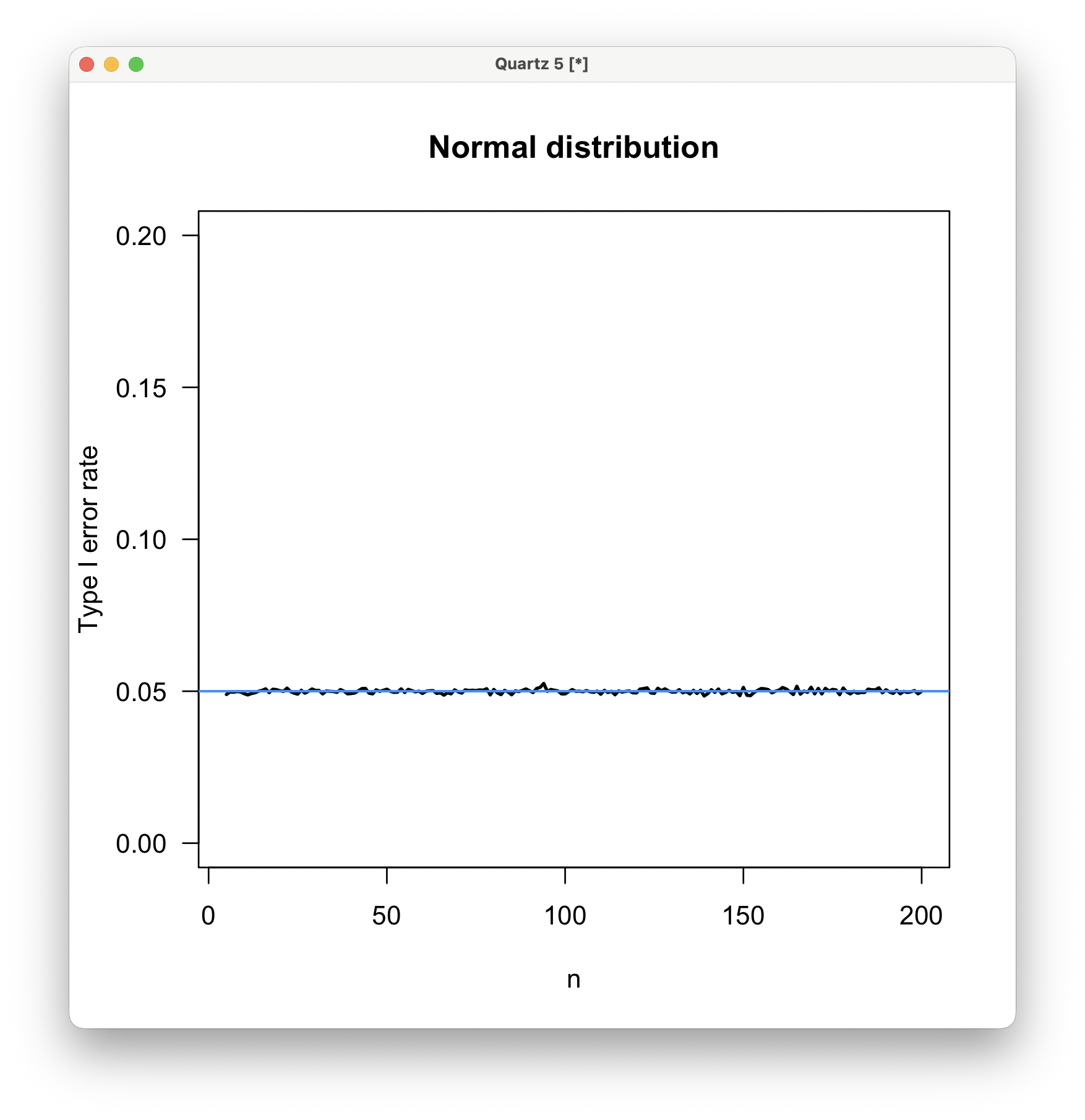
distrib <- rnorm mainTitle <- "Normal distribution" nullHyp <- 0 alpha <- 0.05 numTrials <- 100000 sampleSize <- seq(5, 200, 1) typeIErrorRate <- rep(9999, length(sampleSize)) for (i in 1:length(sampleSize)) { pvalues <- replicate(numTrials, oneTtest(sampleSize[i], FUN=distrib, null=nullHyp)) typeIErrorRate[i] <- sum(pvalues < alpha) / length(pvalues) } dev.new(height=6, width=6) plot(sampleSize, typeIErrorRate, type="l", lwd=2, las=1, main=mainTitle, xlab="n", ylab="Type I error rate", ylim=c(0, 0.20)) abline(h=0.05, col="dodgerblue", lwd=1.5)
Here are the results; the black line is the observed type I error rate, and the blue line is the expected rate (0.05). The type I error rate matches the expectation when the parent distribution is normal, even at sample sizes as small as n=5. The t-test will produce valid results when the data are normally distributed, even at quite small sample sizes.
Exponential distribution
For an exponential distribution, I used the default rexp() function, which has a mean of 1.
distrib <- rexp mainTitle <- "Exponential distribution" nullHyp <- 1 alpha <- 0.05 numTrials <- 100000 sampleSize <- seq(5, 200, 1) typeIErrorRate <- rep(9999, length(sampleSize)) for (i in 1:length(sampleSize)) { pvalues <- replicate(numTrials, oneTtest(sampleSize[i], FUN=distrib, null=nullHyp)) typeIErrorRate[i] <- sum(pvalues < alpha) / length(pvalues) } plot(sampleSize, typeIErrorRate, type="l", lwd=2, las=1, main=mainTitle, xlab="n", ylab="Type I error rate", ylim=c(0, 0.20)) abline(h=0.05, col="dodgerblue", lwd=1.5)
For an exponential distribution, the type I error rate is 11% at n=5, declining rapidly with sample size. By a sample size of 50, the type I error rate is only slightly elevated above the expectation, but it never quite reaches the expected 0.05 value, even at a sample size of 200. Using a t-test on untransformed exponentially distributed data is increasingly inadvisable at sample sizes of less than about 30.

Lognormal distribution
For a lognormal distribution, I use the default rlnorm() function, which has a mean of e0.5.
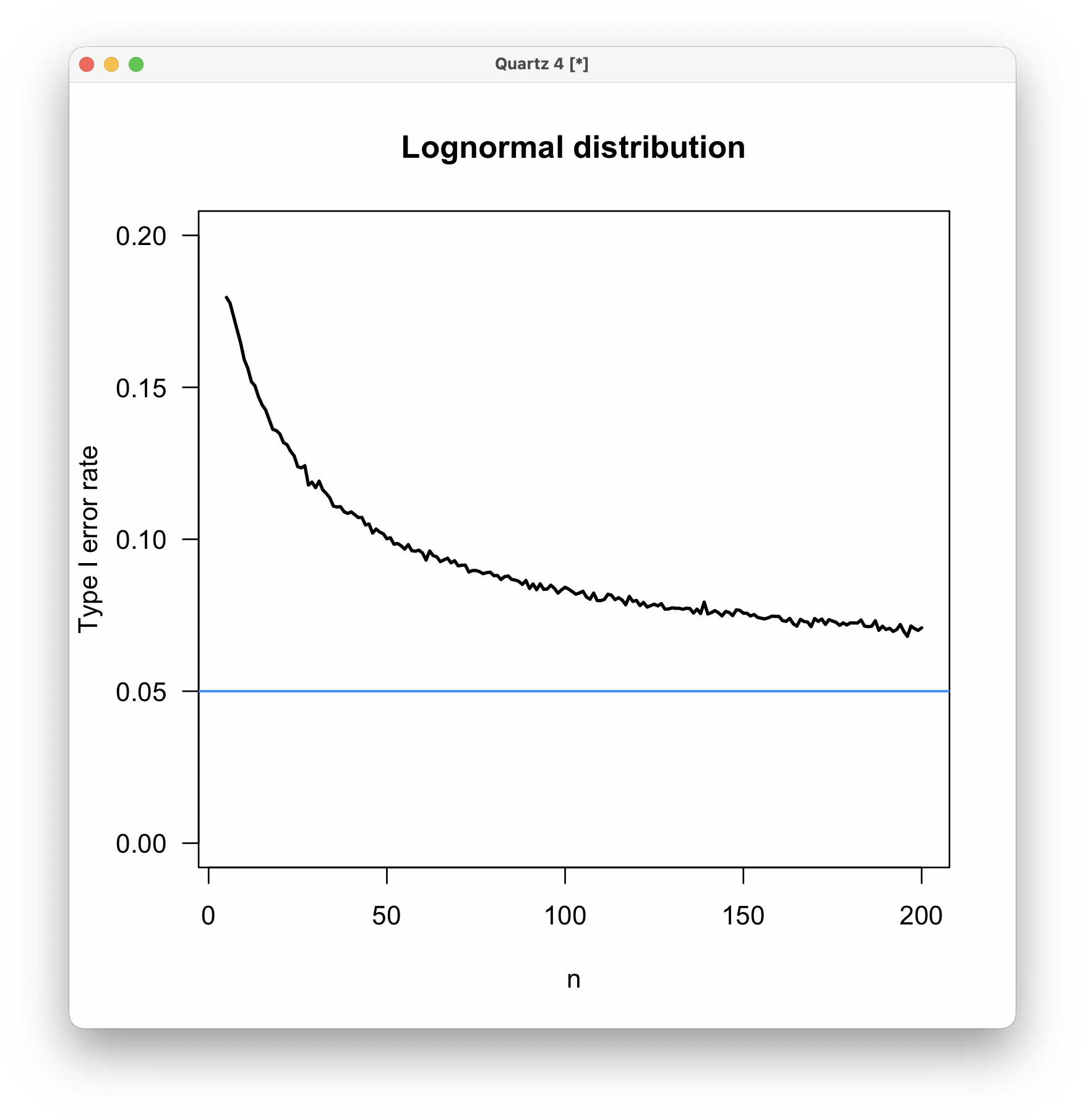
distrib <- rlnorm mainTitle <- "Lognormal distribution" nullHyp <- exp(0.5) alpha <- 0.05 numTrials <- 100000 sampleSize <- seq(5, 200, 1) typeIErrorRate <- rep(9999, length(sampleSize)) for (i in 1:length(sampleSize)) { pvalues <- replicate(numTrials, oneTtest(sampleSize[i], FUN=distrib, null=nullHyp)) typeIErrorRate[i] <- sum(pvalues < alpha) / length(pvalues) } dev.new(height=6, width=6) plot(sampleSize, typeIErrorRate, type="l", lwd=2, las=1, main=mainTitle, xlab="n", ylab="Type I error rate", ylim=c(0, 0.20)) abline(h=0.05, col="dodgerblue", lwd=1.5)
The elevated type I error rate for lognormally distributed data is striking, being as high as 18% when n=5 and remaining at about 7% even at n=200. This was a surprise to me because I would have guessed that an exponential distribution was more unlike a normal distribution than a lognormal distribution would be, given the greater asymmetry of an exponential distribution.
I ran an additional test, in which I applied a log transformation to the data immediately after generating the random numbers from a lognormal distribution. As expected, this converts the data to a normal distribution, and the result is identical to the simulation for the normal distribution shown above. As this result is rather obvious, I do not include the code or the plot.
The message is clear: if you suspect your data is lognormally distributed, you should apply a log transformation before using a t-test at any sample size less than 200 (and probably higher), regardless of whether you are calculating a p-value or a confidence interval.
Conclusions
Although the central limit theorem states that the distribution of sample means converges on a normal distribution as sample size grows, regardless of the shape of the parent distribution, this convergence can be slow. It is particularly slow for the lognormal distribution, which is widespread in the natural sciences.
Although I have argued previously based on more limited tests and the arguments of other authors that one need not be concerned with the parent distribution above sample sizes of 20–30, I no longer recommend that. If the data are clearly non-normally distributed, a data transformation should be applied to bring them closer to normality. If that is unsuccessful or if no suitable data transformation is available, resampling methods or a non-parametric test should be used.
