Ternary Diagrams
30 October 2016
Ternary diagrams are widely used in geology and other sciences to portray the proportions of three items that are constrained to sum to 100%. For example, sandstones are commonly composed of quartz, two main types of feldspar, and various types of rock fragments called lithics, as well as other types of grains. These proportions of these three main components (quartz, feldspar, lithics) can be recalculated such that they sum to 100% and then plotted on a ternary diagram.
R does not come with a built-in ternary diagram function. One is available through the vcd package, but it offers limited customization, so I’ve developed my own set of ternary diagram functions, available here.
Setting up the data
Most of the functions in ternary.r expect either a 3-column data frame or matrix, or a 3-element vector. In both cases, the three elements or columns correspond to what will be plotted at the top, left, and right corners. For example, sandstones are commonly plotted with quartz at the top, feldspar at the left, and lithics on the right, so the three columns would be (in order), quartz, feldspar, and lithics. The rows will correspond to individual samples.
Each row must sum to 100% to be plotted on a ternary diagram. If your data do not, call percentages() to recalculate the percentages so that they do.
Here is how an example data set might be set up. Note that the call to percentages() isn’t necessary, since the rows already sum to 100%.
q <- c(100, 20, 40, 40, 0, 0, 33.3, 70) f <- c( 0, 40, 20, 40, 100, 0, 33.3, 15) l <- c( 0, 40, 40, 20, 0, 100, 33.3, 15) x <- cbind(q, f, l) x <- percentages(x)
Creating a basic ternary plot
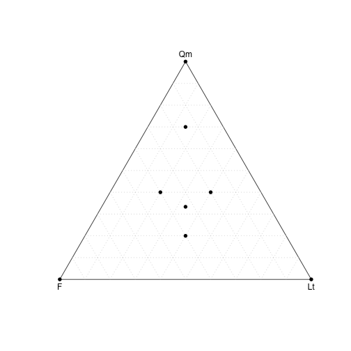
The ternaryPlot() function is always the starting point for making a ternary plot. The first argument is the data set as a matrix or data frame. The labels parameter is a three-element vector for the labels that will appear at the top, left, and right corners. The light gray grid can be turned off by setting grid=FALSE, and the spacing of the grid lines can be set by changing the increment argument, which is the spacing of the grid lines in percentage points. Additional arguments like pch and col can be specified to control the color and type of points to be plotted. For custom plots with added line segments and polygons, the display of points can be turned off by setting plotPoints=FALSE.
ternaryPlot(x, labels=c("Qm", "F", "Lt"), increment=10, pch=16)
Adding points to a plot
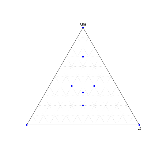
To add points manually, either all at once or in series that have custom characters or colors, use the ternaryPoints() function for each set of data to be added. As with ternaryPlot(), additional parameters like pch and col can be passed to control the appearance of the plotted points.
ternaryPlot(x, labels=c("Qm", "F", "Lt"), increment=10, plotPoints=FALSE) ternaryPoints(x, pch=16, col="blue")
Adding a line segment to a plot
Line segments can be added to the plot with the ternarySegment() function, which takes two arguments, the starting point and end point of the line segment. Additional graphical parameters like lty, lwd, and col can be supplied to customize the segment. Some rock classifications divide the ternary diagram into areas, and ternarySegment() can be used to show those divisions.
ternaryPlot(x, labels=c("Qm", "F", "Lt"), increment=10, pch=16) end0 <- c(70, 15, 15) end1 <- c( 0, 50, 50) ternarySegment(end0, end1, col="red", lwd=2)
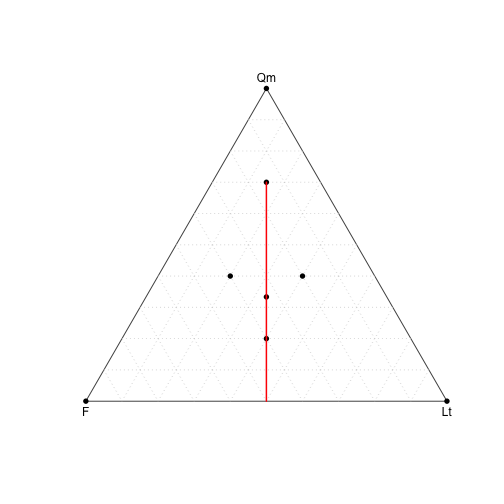
Note that, because the line was added after the points in this example, it covers them. To prevent this, call ternaryPlot() with plotPoints=FALSE, then ternarySegment(), then ternaryPoints(), as shown in the following example for a polygon.
Adding a polygon to a plot
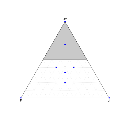
Polygons can be added with ternaryPolygon(), which accepts a matrix of the vertices of the polygon, in either clockwise or counterclockwise order. The first and last vertices should be the same point so that the polygon is closed. The color and border of the polygon can be customized by passing the additional arguments that polygon() would accept.
Because shaded polygons will cover over any points, it is important to plot the points after the polygons are added. This is best done in three steps. First, ternaryPlot() is called with plotPoints=FALSE, followed by all the calls to ternaryPolygon(). Last, all of the calls to ternaryPoints() are made to place the points on top of the plot.
ternaryPlot(x, labels=c("Qm", "F", "Lt"), increment=10, plotPoints=FALSE) a <- c(100, 0, 0) b <- c( 50, 50, 0) c <- c( 50, 0, 50) poly <- rbind(a, b, c, a) ternaryPolygon(poly, col="lightgray") ternaryPoints(x, pch=16, col="blue")
Adding text to a plot
Text can be added with ternaryText(), which takes the position of the text, the string to be displayed. Additional graphical parameters to style the text, such as its color, position or font, the same as would be used in the text() function on a scatterplot.
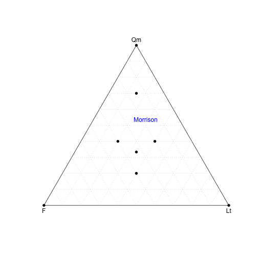
ternaryPlot(x, labels=c("Qm", "F", "Lt"), increment=10, pch=16) coords <- c(50, 20, 30) ternaryText(coords, "Morrison", col="blue", pos=3)
Code files
Comments
Comments or questions? Contact me at stratum@uga.edu
