BIRD-SONG SONOGRAMS IN R
05/14/2017
I’ve birded for many years, and one of my goals this summer is to learn to bird by ear. After starting the Cornell Lab of Ornithology course on How to Identify Bird Songs, I’ve become sold on sonograms, pictorial representations of bird songs that show the frequency of the song through time. They’re easy to make with a cell phone and R, and that’s what I’ll show here.
There are two steps in this process: recording the sounds, and constructing the sonogram.
Recording the sounds
I recommend the app Røde Rec for recording bird calls. It makes it easy to record and export, although it took a bit of experimentation to learn how to trim and edit the sound clip.
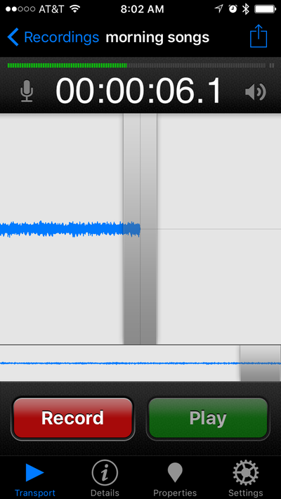
To record a bird call, create a new recording, press record to start, then stop when you’re finished. The iPhone and iPad microphones aren’t ideal for recording bird calls, partly because they’re meant to record close-up sounds, like your voice. To get the best results, point the microphone toward the bird, and stay perfectly still and quiet while recording. Whatever noises you make will drown out the bird sounds that are recorded.
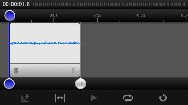
You will likely want to edit your recording to trim away sounds before and after the song you’re interested in, and Røde Rec has editing tools built in. They’re always visible in the iPad app, but you’ll need to rotate an iPhone to landscape to see them. The main controls you need to use are the handles (circled in yellow) and the drag bar (circled in orange).
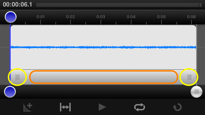
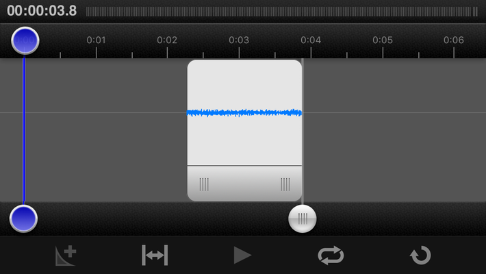
First, drag the handles to encompass just the part of the sound you want to save.
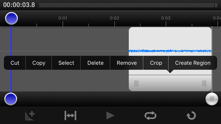
Next, press and hold on one of the handles to bring up a menu, then tap on crop in that menu.
Tap and drag on the drag bar to bring the selected sound all the way to the left, to the beginning of the time line.
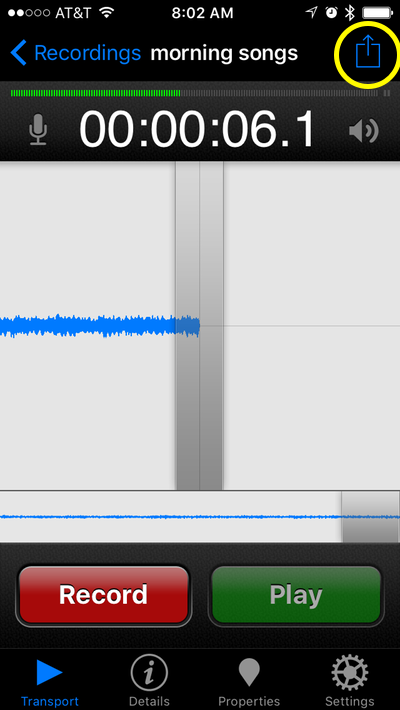
To export your sound, return the iPhone to portrait mode and tap the share button in the upper right (circled in yellow, below). Select how you would like to export and follow the instructions. I chose email, and that worked fine.
Last, put the file on your Mac where you can easily retrieve it from R, usually whatever working directory you use in R.
Constructing the sonogram
First, install and load the two libraries you need to read the .wav sound file (tuneR) and construct the sonogram (seewave).
library(seewave)
library(tuneR)
Load the sound file (as a .wav file) that you exported from Røde Rec; mine is a clip of a Prothonotary Warbler calling from our river bank. Display the data for the sound file to see the details of the recording.
protho <- readWave("prothonotaryWarbler.wav")
protho
Doing this reveals the basic structure of the sound recording, including the duration and sampling rate. Because the sound rate is embedded in the file, we will not have to specify it when we draw the spectrogram. Note also that the iPhone records in mono, not stereo, and that it records 24-bit sound.
Wave Object
Number of Samples: 3247517
Duration (seconds): 67.66
Samplingrate (Hertz): 48000
Channels (Mono/Stereo): Mono
PCM (integer format): TRUE
Bit (8/16/24/32/64): 24
Making the sonogram of the full sound clip takes a single command, spectro(). To show the oscillogram below the sonogram, add osc=TRUE. The oscillogram gives a good picture of the loudness of the sounds.
spectro(protho, osc=TRUE)
Chances are, your clip is longer than the sounds you’re interested in. In the sonogram, note the times of the beginning and the end of the interesting sounds, then read just that portion of the sound file and make a new sonogram from it.
protho1 <- readWave("prothonotaryWarbler.wav", from=56, to=58, units="seconds")
spectro(protho1, osc=TRUE)
protho2 <- readWave("prothonotaryWarbler.wav", from=63, to=66, units="seconds")
spectro(protho2, osc=TRUE)
Here’s what these two look like.
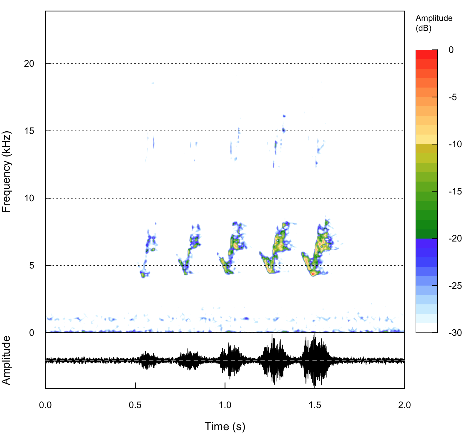
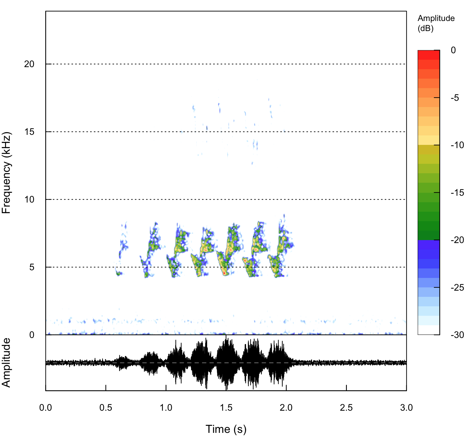
The top part of each plot shows the sonogram, with time going from left to right, and frequency increasing upward (that is, low pitches near the bottom and high pitches near the top). The color scale indicates the intensity of that frequency. These plots show that the song consists of 5–7 repeated notes, each of which gets lower in pitch then higher in pitch.
The oscillogram is shown at the bottom of each plot, and it indicates the loudness of the call through time. In the first recording, the loudness builds with each note, and in the second, it builds through the first five, then declines in the last two.
Sonograms like these give a good picture of what the bird is singing and can help you visualize and remember bird calls.