Randomization and the number of trials
17 July 2025
Resampling methods, including randomization, Monte Carlo, bootstrap, and jackknife, are common ways of generating confidence intervals and p-values. They are often employed when the underlying distribution is unknown, such that common parametric methods like the t-test cannot be used.
The results of these methods are sensitive to the number of resampling trials. For example, confidence limits or p-values might change from one run of the resampling method to another. How much they change can depend greatly on the number of resampling trials. Here, I’ll illustrate this by using randomization to estimate the p-value of a correlation coefficient.
An example: p-value of a correlation coefficient
Imagine we have measured two variables, x and y, shown below.
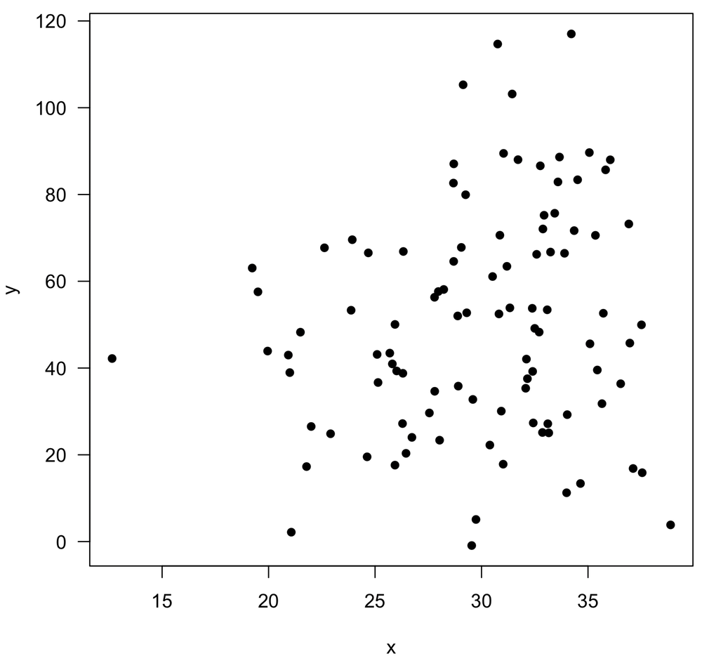
We calculate a correlation coefficient of 0.16, and we would like to generate a p-value for it. Rather than do this the usual way by running a t-test of the correlation coefficient where our null hypothesis is that the correlation is zero (done with cor.test()), we decide to use randomization.
As a side note, I wouldn’t recommend this approach to the problem. I am using it just to demonstrate the overall concept of the effect of the number of randomization trials.
Randomization of the correlation coefficient would work like this. We would take the y-values and scramble their order, so that they are no longer correctly paired with the x-values, and we would calculate a correlation coefficient. It should be obvious that every time we do this, we will get a somewhat different randomized correlation coefficient. Our question becomes “How unusual is our observed correlation coefficient of 0.16 compared with these randomized coefficients?” We evaluate that by doing this randomization 100 times (trials), seeing how often we get a randomized correlation coefficient greater than what we observe. We divide this count by the number of randomization trials, and that gives us a p-value of 0.07.
For curiosity, we try this again by performing another 100 trials, but this time we get a p-value of 0.06. Uh oh, it’s the value is different. We try again: 0.06. And again: 0.08. And again: 0.03. This is worrisome: our p-value is not stable; it’s not repeatable.
We decide we want to see how bad the problem is so we run our experiment 1000 times, that is, we perform 1000 separate experiments, where in each, we generate 100 randomized r values from which we will calculate a p-value. Remember, the number of randomized r values used to calculate a p-value is the number of trials (100), not the number of times we repeat the entire process (1000) to see how p is distributed. We plot the distribution of p-values, and it looks like this:
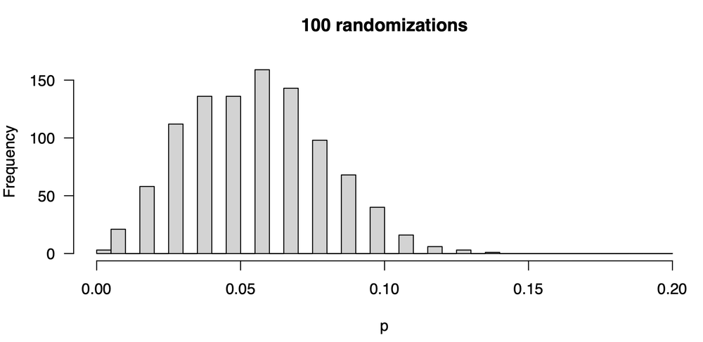
The first thing we notice are the gaps. If we have 100 randomization trials, only certain p-values can result: 0, 0.01, 0.02, 0.03, etc.— nothing in between is possible, so we get gaps in our frequency distribution. The second thing we notice is that any given attempt at calculating a p-value could give us quite different results: we might have gotten a p-value as low as zero or as large as 0.14, and that could lead us to quite different conclusions. Moreover if we are overly focused on a p-value of 0.05 (as you should not be), sometimes we will see a statistically significant correlation and sometimes we won’t.
The solution is to increase the number of randomization trials. Instead of 100, we raise it ten-fold to 1000. In each experiment, we shuffle our y-values 1000 times instead of 100 and calculate a correlation coefficient. From those 1000 values we calculate a p-value. Here’s what the distribution of p-values now looks like:
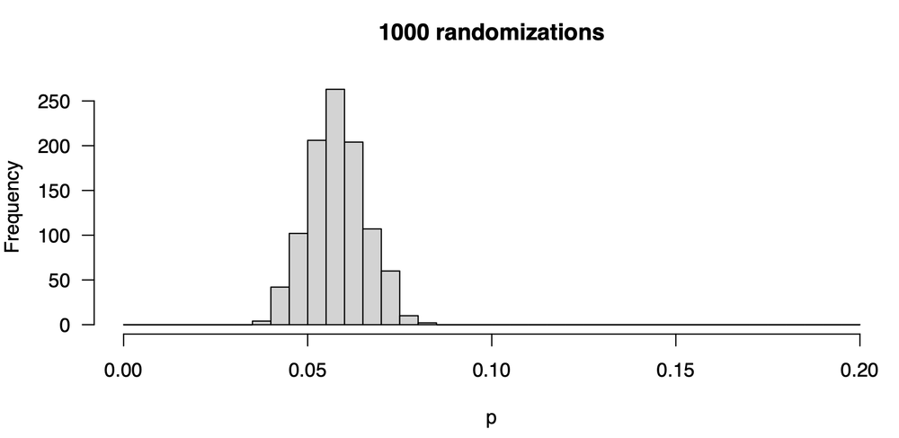
This is better: our p-values are more stable: we are less likely to get very large or small values. Still, they vary: some are as low as 0.04, and some are as high as 0.085. Notice that the central tendency hasn’t shifted from our first attempt: the values tend to be around 0.06. The central tendency hasn’t changed, but the distribution—our uncertainty in the p-value— has decreased. Let’s increase the number of trials ten-fold from 1000 to 10000; here is the new distribution of p-values:
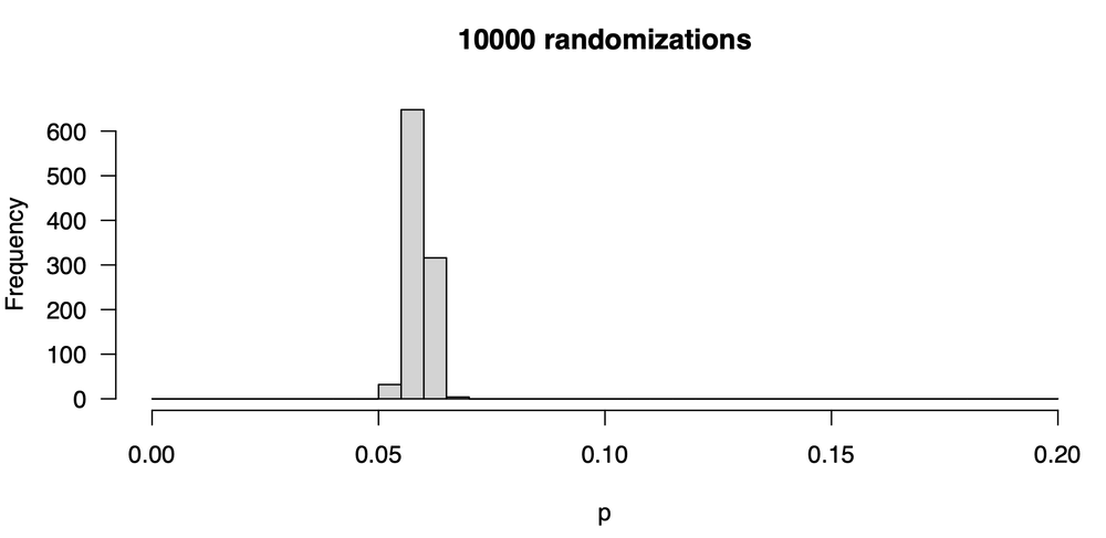
This is a marked improvement, as there is much less variability in our p-value from one trial to the next. The values are all around 0.06; some are as low as 0.055 and a few are as high as 0.070. Let’s go one step further, increasing the number of trials ten-fold to 100,000. Here is the distribution of p-values:
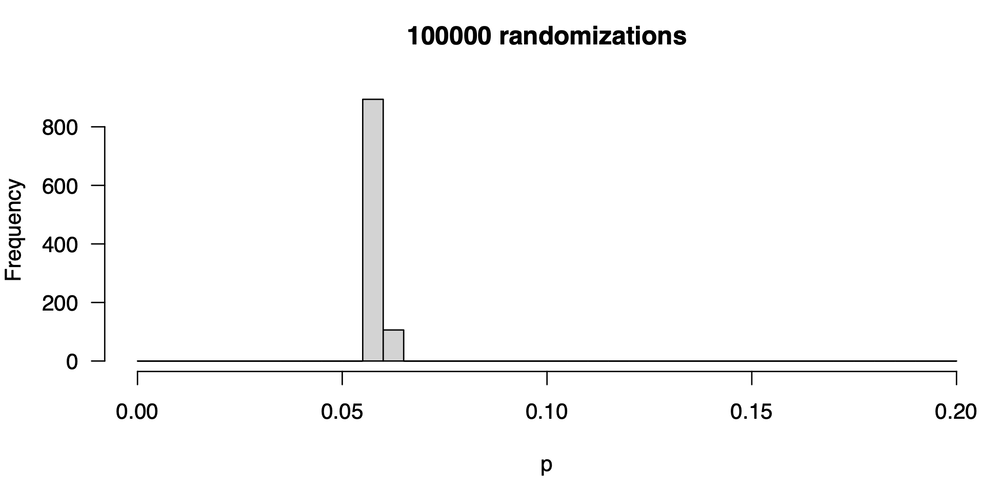
This is quite tight, and nearly all the p-values are 0.06. What you should realize is that the stability of the p-value you report is strongly controlled by the number of randomization trials. The p-value will always vary somewhat in any resampling method, but you want the variation to be trivial, unimportantly small. You do that by raising the number of trials.
The cost
You might be wondering why you shouldn’t just make the number of trials extremely large, say, 10 billion. That would usually make your p-value quite stable, but the cost is run time. Resampling methods can be time-intensive, particularly for some problems. The run times aren’t great in this example. Calculating one p-value for 100 trials here takes 0.148 seconds, 1000 trials takes 0.0288 seconds, 10000 trials takes 0.165 seconds, and 100000 trials takes 1.486 seconds. You might expect every 10-fold increase in the number of trials would increase the run time by a factor of 10. That’s a good guideline, although it isn’t always true (for example, going from 100 to 1000 trials in this example only doubles the run time).
Of course, the run times in this example are so short that you could make the number of trials gigantic without much of a penalty. Beyond a certain point, though, increasing the number of trials doesn’t help much. For example, 100,000 trials is plenty in this case. Going to 1,000,000 trials would make the p-value a little more stable, but that won’t have a practical effect. (For example, we would never want to split hairs over whether a p-value was 0.049 or 0.051.) At a certain point, increasing the number of trials is wasted precision.
For some problems, the run time for calculating one p-value might be long, hours to days or even more, so there will be limits to how many trials can be reasonably done. Realize that there are tradeoffs in your precision and your run time, and you will need to find a balance.
How many trials should I do?
There is no simple answer to this question, and the answer will depend on the tradeoff between precision and run time.
Typically, I start with an unreasonably small number of trials (for example, 10) to get a sense of run time. Once I know that, I estimate how long I want my first estimate to take, and I use that to calculate how many trials I will need. For example, let’s say I am comfortable with a one-hour run; I can make a rough estimate of the number of trials. Once I get that estimate, I run the code again to get a second p-value (or confidence interval), and then a third, similar to the thought experiment we did above. If the results are stable, I will go with that, but if there’s substantial variation, I will raise the number of trials by a factor of 10 as we did here until the results are stable enough for my needs.
I rarely not repeat the process 1000 times as I did in these examples to generate a distribution of p-values or confidence intervals. It is much more useful to spend computing time by increasing the number of trials to produce a single stable p-value or confidence interval than to generate distributions of those values. For example, generating that last plot (100,000 randomization trials done 1000 times) took 24.4 minutes, but 1,000,000 randomization trials done once took only 14.4 seconds. Repeating that three times gave me p-values of 0.0592, 0.0594, 0.0589, effectively the same value and certainly not different enough to lead to different conclusions.
Code for this simulation
The code for generating this post and its plots is included below.
# Simulate some data x <- rnorm(100, mean=30, sd=5) y <- 1.3 * x + 12.2 + rnorm(100, sd=30) plot(x, y) rObserved <- cor(x, y) # Function to shuffle the y-values and calculate the randomized # correlation coefficient oneTrial <- function(x, y) { yShuffled <- sample(y, length(y)) cor(x, yShuffled) } # Force same scales on frequency distributions of p-values breaks <- seq(0, 0.2, 0.005) # Run 1000 p-value simulations of 100 randomizations each startTime <- Sys.time() numRandomizations <- 100 numSimulations <- 1000 p <- rep(-9999, numSimulations) for (sim in 1:numSimulations) { rShuffled <- replicate(numRandomizations, oneTrial(x, y)) p[sim] <- sum(rShuffled > rObserved) / numRandomizations } fileName <- paste(numRandomizations, "randomizations.pdf", sep="") pdf(fileName, height=4, width=8) plotTitle <- paste(numRandomizations, " randomizations", sep="") hist(p, breaks=breaks, main=plotTitle, las=1) Sys.time() - startTime dev.off() # Run 1000 p-value simulations of 1000 randomizations each startTime <- Sys.time() numRandomizations <- 1000 numSimulations <- 1000 p <- rep(-9999, numSimulations) for (sim in 1:numSimulations) { rShuffled <- replicate(numRandomizations, oneTrial(x, y)) p[sim] <- sum(rShuffled > rObserved) / numRandomizations } fileName <- paste(numRandomizations, "randomizations.pdf", sep="") pdf(fileName, height=4, width=8) plotTitle <- paste(numRandomizations, " randomizations", sep="") hist(p, breaks=breaks, main=plotTitle, las=1) Sys.time() - startTime dev.off() # Run 1000 p-value simulations of 10000 randomizations each startTime <- Sys.time() numRandomizations <- 10000 numSimulations <- 1000 p <- rep(-9999, numSimulations) for (sim in 1:numSimulations) { rShuffled <- replicate(numRandomizations, oneTrial(x, y)) p[sim] <- sum(rShuffled > rObserved) / numRandomizations } fileName <- paste(numRandomizations, "randomizations.pdf", sep="") pdf(fileName, height=4, width=8) plotTitle <- paste(numRandomizations, " randomizations", sep="") hist(p, breaks=breaks, main=plotTitle, las=1) Sys.time() - startTime dev.off() # Run 1000 p-value simulations of 100000 randomizations each startTime <- Sys.time() numRandomizations <- 100000 numSimulations <- 1000 p <- rep(-9999, numSimulations) for (sim in 1:numSimulations) { rShuffled <- replicate(numRandomizations, oneTrial(x, y)) p[sim] <- sum(rShuffled > rObserved) / numRandomizations } fileName <- paste(numRandomizations, "randomizations.pdf", sep="") pdf(fileName, height=4, width=8) plotTitle <- paste(numRandomizations, " randomizations", sep="") hist(p, breaks=breaks, main=plotTitle, las=1) Sys.time() - startTime dev.off() # Calculate the time it takes to run one randomization trial. numRandomizations <- 100 startTime <- Sys.time() rShuffled <- replicate(numRandomizations, oneTrial(x, y)) Sys.time() - startTime numRandomizations <- 1000 startTime <- Sys.time() rShuffled <- replicate(numRandomizations, oneTrial(x, y)) Sys.time() - startTime numRandomizations <- 10000 startTime <- Sys.time() rShuffled <- replicate(numRandomizations, oneTrial(x, y)) Sys.time() - startTime numRandomizations <- 100000 startTime <- Sys.time() rShuffled <- replicate(numRandomizations, oneTrial(x, y)) Sys.time() - startTime
